Object Tracking with OpenCV
Overview
In this tutorial we’re going to add another kind of autonomy to our robot, and that’s object tracking with the camera. Also known as visual servoing this is where we use the camera to detect a key object, then based on where it is in our field of view we send an appropriate control signal for the robot to follow it.
This algorithm has two parts, split into two nodes. One handles all the detection/image processing (using OpenCV to look for our object and return its coordinates within the camera frame) and the other handles the "following" (taking the detection measurement and calculating the command velocity to send to the control system).
We'll demonstrate this first in simulation, and then on the real robot. The detected object for this example will be a tennis ball, but you could take this concept and apply it to faces, another robot, or anything else you can detect.
Pre-work
Install OpenCV
This project uses OpenCV (via Python) to perform image detection, we can install this with:
sudo apt install python3-opencv
Fix up twist_mux
One little thing I’m going to do to begin with, that we’ll need later in the tutorial, is to update our twist_mux config yaml. We’re adding a new source of command velocity so let’s copy one of the other ones. I’ll set the priority somewhere similar to the navigation one.
ball_tracker:
  topic   : cmd_vel_tracker
  timeout : 0.5
  priority: 20
We’ll just have to make sure we remember to remap the output command velocity topic to match this name when it comes time.
Preparing the simulation
Previous versions of this tutorial, for the old Gazebo, walked through the process of creating a yellow tennis ball model in Gazebo. This is more difficult in the new Gazebo, since there is currently no scale tool and there are also sometimes issues changing the colour of objects.
Before we can detect our ball, we need to simulate it. We’ll start by running our Gazebo launch file, just like the previous tutorials (e.g. ros2 launch my_bot launch_sim.launch.py).
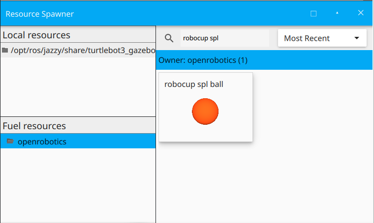
We will add an existing ball model. Using the Resource Spawner, search for robocup spl ball, click the download icon, and once downloaded you can click the thumbnail and move your mouse over the 3D view to spawn the ball. It may spawn in the ground, in which case you can use the move tool to move it into the air and drop it.
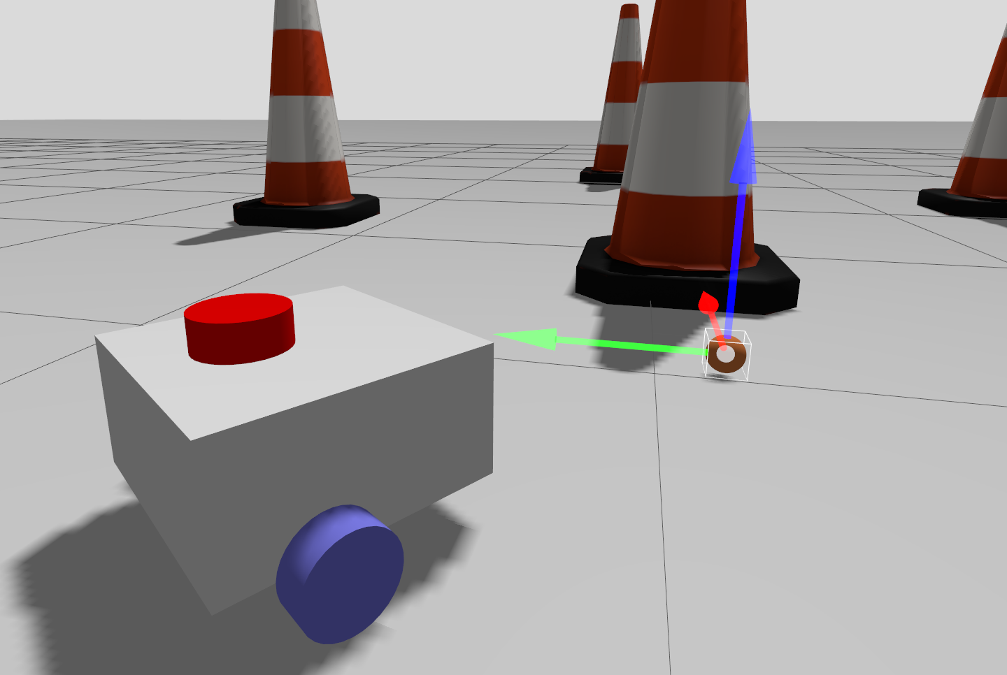
Now, if we drive our robot around we should see the ball in RViz (you can add an Image or Camera panel and set the topic if you haven't already).
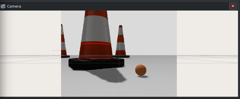
The other thing we might want to do is to tilt the camera down just a little so that it sees the ground better. In camera.xacro we want to adjust the pitch of the camera_joint (I used 0.18 radians for the example below), and rerun the simulation.
1
Cloning the ball_tracker repo
Clone the ball_tracker repo from here into your workspace and rebuild.
cd ~/dev_ws/src
git clone https://github.com/joshnewans/ball_tracker.git
cd ..
colcon build
The code is heavily based on a ROS 1 tutorial by Tiziano Fiorenzani so if you want to know more details you can go ahead and check that out. His code is also available here.
Detecting the Ball
Now that we’ve got our camera seeing the ball, the first node we need is one for detecting it. We want this node to take the raw image in, pick out the ball, and return its location within the image frame on the /detected_ball topic. There are also some Image topics used to assist with tuning and monitoring the algorithm.
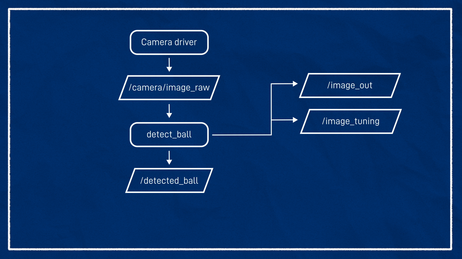
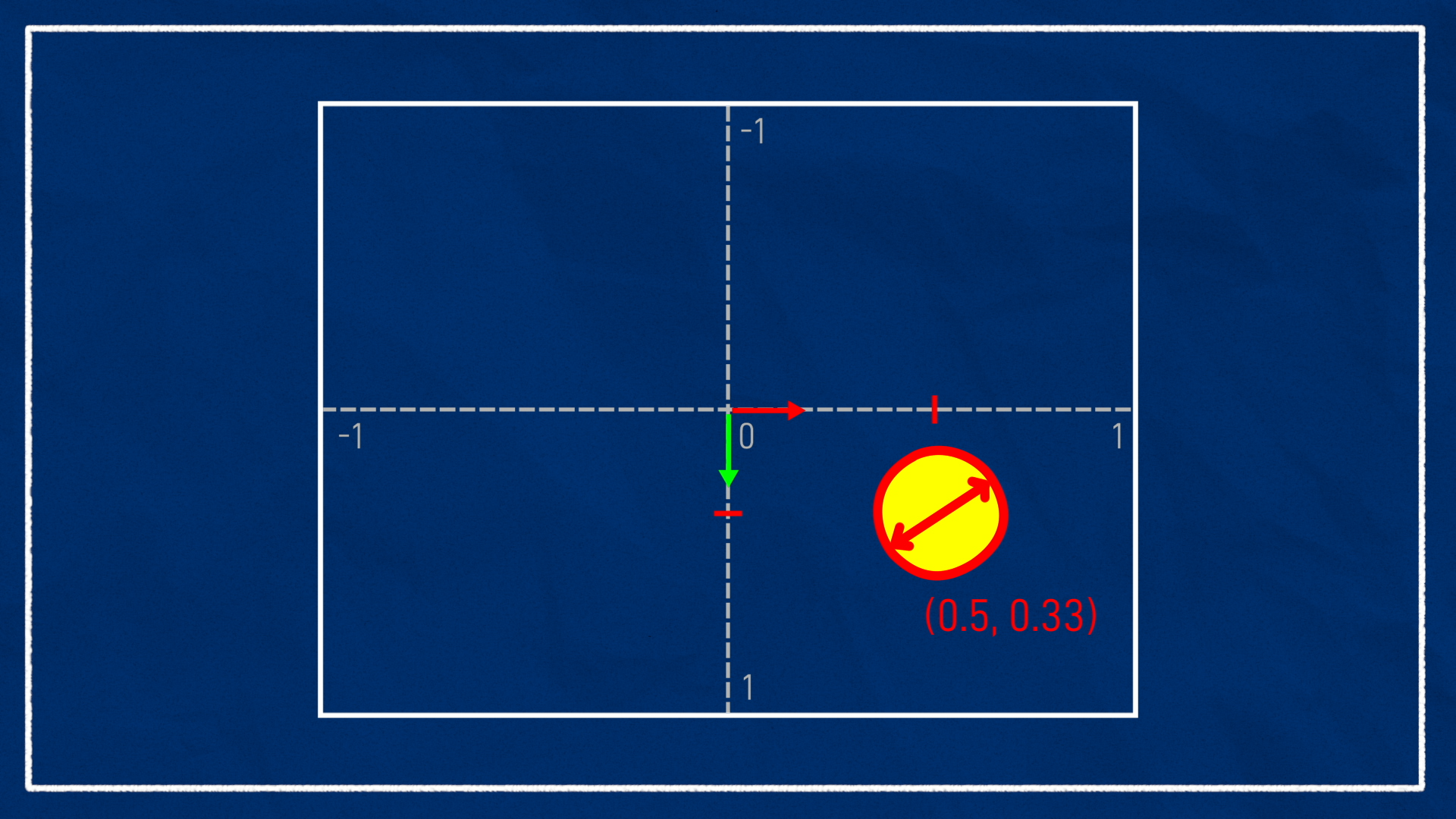
We’re going to have the centre of the frame be (0,0), and the frame edges be 1. Remember that the optical frame has X right and Y down. So a ball 3/4 across and 2/3 down from the top-left corner will have a position of (0.5, 0.33). We’ll return the diameter of the detected ball as the Z value, as a fraction of the frame width. So a ball that is half as wide as the frame will have a Z value of 0.5.
Running the node
The node we want to run first is detect_ball. By default it is expecting a bunch of tuning parameters to be passed in, but we don’t know them yet, so we’re going to set tuning_mode to true. This will pop up with a little window of sliders to help us tune. The other thing we want to do is remap the image_in topic to /camera/image_raw to match our simulated camera output.
ros2 run ball_tracker detect_ball --ros-args -p tuning_mode:=true -r image_in:=camera/image_raw
Tuning the detection
To tune the detection, we want to open a new Image display in RViz, and set the topic to /image_tuning. This will show us what the algorithm is thinking. At the moment it should look the same as our input.
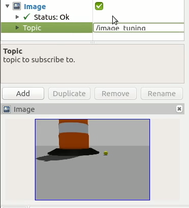
Now we want to place the ball in front of the robot and adjust the tuning parameters using the sliders, until the ball is detected as reliably as possible. The behaviour of the parameters is described below:
- X (min/max) - The horizontal limits to search for the ball (percentage left to right).
- Y (min/max) - The vertical limits to search for the ball (note that the min is at the top and max is at the bottom, this is common in image processing).
- Hue (min/max) - The hue limits. This is probably the most important parameter, as it is how we isolate a particular colour (e.g. red, yellow, green).
- Sat (min/max) - The saturation limits. This is how rich/vibrant the colour is.
- Val (min/max) - The value limits. This is how light/dark the colour is.
- Size (min/max) - The size limits in percent of screen size.
Detecting a red hue is more difficult as it is at the "wrap-around". This can be achieved by applying multiple filters or doing some clever shifting of the image colours. Either way, it requires a bit of extra code.
One way to get a feel for these parameters is to add a "Spectrum Plane" into the scene. If we put it somewhere the camera can see it well, we can see the effects of varying each parameter. While this worked well in the old Gazebo, it does not seem to load correctly in the current version.
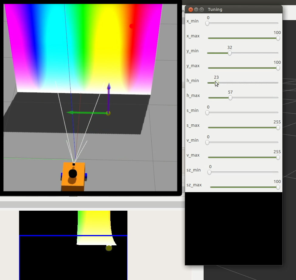
Once the parameters have been tuned and the ball is isolated, we can switch to the output view by changing the topic to /image_out, and we should see the whole image with the ball location indicated.
As an example, I am using a tennis ball, so I have isolated a yellow/lime kind of hue. My robot is on the ground and the ball will be on or near the ground, so I have reduced the Y limits. Some of the other parameters have been adjusted to suit.
My parameters:
X: 0-100 (Use the whole width)
Y: 32-100 (Ignore above the horizon)
Hue: 8-19 (Tight range around orange)
Saturation: 133-255 (Needs to be reasonably saturated but not lose all shadows)
Value: 50-230 (Avoid very white or black areas)
Size: 0-25 (Try to avoid misclassifying large objects)
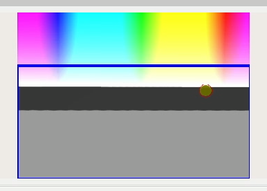
The primary output of this node is the location of the detected ball, so we echo /detected_ball and remember X is from -1 on the left to 1 on the right, and Y is -1 at the top to 1 at the bottom, with 0,0 being the centre and Z is the ball diameter as a fraction of the frame width.

Have a go at dragging the ball to different locations while monitoring the various outputs.
At this point we should write down our tuning parameters. Later on in the tutorial we’ll be putting them into a params file so that we can load them back up again easily, but for now we’ll just leave it running in tuning mode.
Advanced Tracking
There are plenty of more advanced things we could do in terms of detection, here is just one brief example.
As humans, we know that the further away an object is, the smaller it looks. Given this, if we know the true size of the ball, and the characteristics of the camera, we should be able to roughly determine the location of the ball in real space.
If we were doing this seriously, there is a great method that involves calibrating our camera, compensating for distortion, etc, but since this is just a beginner’s example we use a simpler based on standard trigonometry, as per the image below.
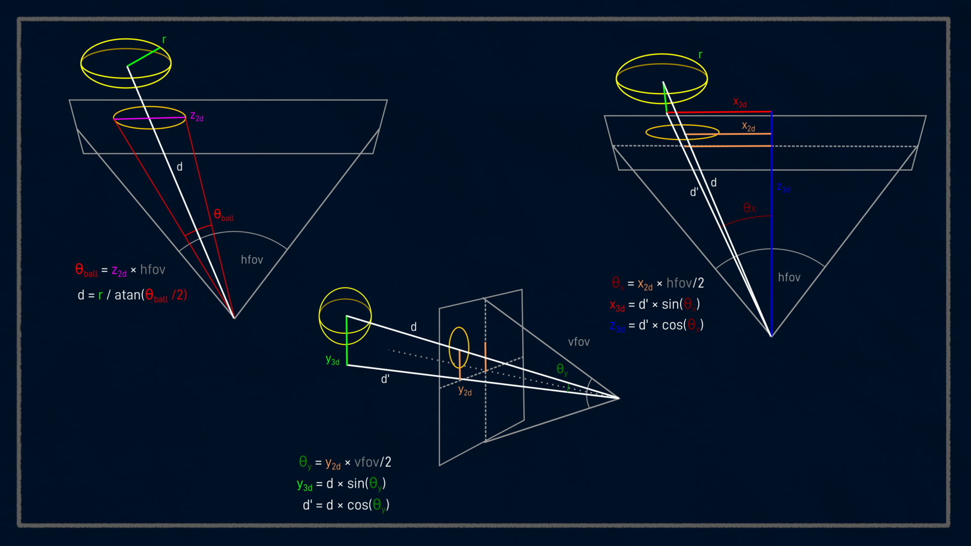
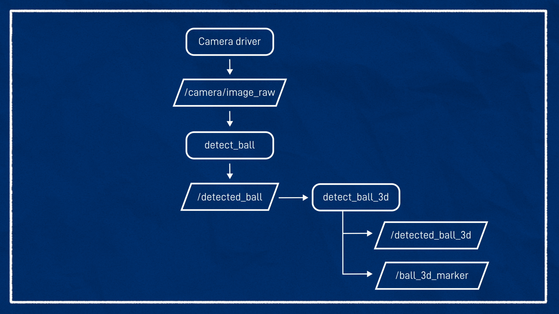
The ball_tracker package contains a node detect_ball_3d to perform these calculations. It will subscribe to /detected_ball and publish the 3D point to /detected_ball_3d. It will also publish a Marker topic for RViz, at /ball_3d_marker. We can run the node by simply entering: ros2 run ball_tracker detect_ball_3d.
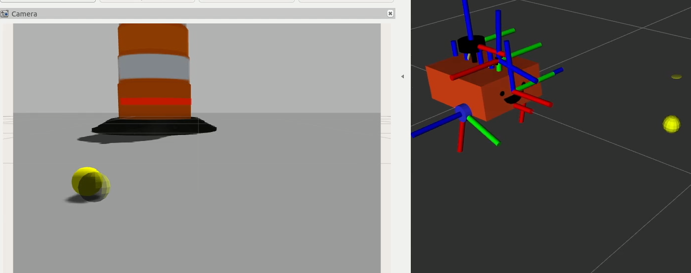
After adding the marker to RViz, we should see the ball appear in the 3D view. If we also add a Camera display (not Image), we should see the 3D estimate overlaid over our camera feed. It's not too bad!
Following the ball
Now we need to tell the robot to follow the ball. The follow_ball node that we’ll run is pretty simple, conceptually.
- When it can’t see a ball, the robot will spin in circles until it finds one
- Once it sees the ball, the angular speed will be set proportional to the distance the ball is away from the centre, so full speed if the ball is right at the edge of the camera frame, and no rotation if it’s in the centre
- The forward speed will be set to a constant if the ball is too far away (i.e. too small in the frame), and once it is close enough (or big enough), the forward speed is set to 0 to ensure we don’t run over it.
The provided implementation just uses the "2D" /detected_ball, but a great exercise would be to copy the node and creating a similar control strategy utilising the estimated 3D ball location!
Remember when we run this, we want to remap the command velocity as per our twist_mux config.
ros2 run ball_tracker follow_ball --ros-args -p use_sim_time:=true -r cmd_vel:=cmd_vel_tracker
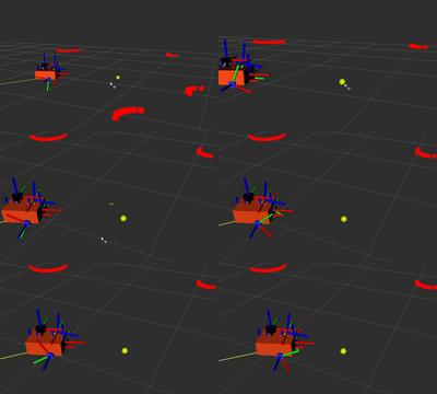
In the Gazebo (or RViz) window we should see the robot begin to move and follow the ball! Try dragging the ball to different locations and see if the robot can find it!
Just as with the detection node, this node has some parameters we can tweak, so let's take a closer look at them.
Config Parameters and Launch File
Like the nodes from earlier tutorials, it's convenient to tidy all these parameters up into a file. The ball_tracker repo comes with an example for us (config/ball_tracker_params_example.yaml) so let's copy that file into our own config directory, and rename it ball_tracker_params_sim.yaml (we'll have slightly different parameters for the simulation and the real robot due to differences in the camera image).
The contents of the example (which include all the parameters we can tweak) are shown below:
1
At this point we could run the nodes again and pass the params file in to each of them, but it's better to use a launch file!
The ball_tracker repo comes with its own launch file that bundles up all the nodes and exposes some handy launch arguments. To see all the available arguments we can type:
ros2 launch ball_tracker ball_tracker.launch.py --show-args
detect_only- Defaults to false, doesn’t run the follow component. Useful for just testing the detectionsfollow_only- Defaults to false, you guessed it, good for testing just the follow component (you’d publish the detection message manually)tune_detection- Enables tuning mode for the detectionuse_sim_time- (Currently unused) Tell the nodes to use Gazebo simulated timeimage_topic- The name of the input image topic. Default/camera/image_rawcmd_vel_topic- The name of the output command vel topic. Default/cmd_vel_trackerenable_3d_tracker- Defaults to false, enables the 3D tracker node
So to replicate our previous behaviour, could run something like...
ros2 launch ball_tracker ball_tracker.launch.py params_file:=path/to/params.yaml image_topic:=/camera/image_raw cmd_vel_topic:=/cmd_vel_tracker enable_3d_tracker:=true
Because even that is a bit of a mouthful to remember, we can create our own launch file in our main project repo and include the ball_tracker one. The ball_tracker repo contains an example of this in launch/example_launch_include.launch.py to copy and modify.
1
Real camera
Now that we’ve got it all working in simulation, let’s try it on the real robot. Here we have two options:
- Run the whole pipeline on the robot
- Run the
ball_trackernodes on the base station/dev machine
Because it uses ROS topics for input and output, either will work! The sections below explain how to run the detection on a different machine, as there are some extra steps we need to take to avoid a major performance hit.
Run Camera Driver and Fix image topic
Before we launch our camera driver, we want to edit our launch file (e.g. camera.launch.py) and add a namespace of 'camera'. This will ensure our real camera behaves more like our simulated camera, putting the image in a namespace.
executable='v4l2_camera_node',
             output='screen',
             namespace='camera',
             parameters=[{
                 'image_size': [640,480],
                 'time_per_frame': [1, 6],
                 'camera_frame_id': 'camera_link_optical'
                 }]
Note, compared to the initial camera setup tutorial, I have also customised the camera frame rate which is in
time_per_frameas a fraction of a second (numerator and denominator).
Then, we can run our camera driver like normal (e.g. ros2 launch my_bot camera.launch.py).
Republish topic on dev machine
When we’re performing image processing on the dev machine, we don’t want to bog down the Wi-Fi by streaming the raw image feed over the network. Instead, we want to use a compressed image. Our camera driver already publishes a compressed image which is great, but since the ball detector is written in Python and Python nodes don’t play nicely with compressed images, we’re going to run a republish node on the dev machine to decompress it once it's over the network. Just be aware that this means we need to also adjust the image topic we are remapping.
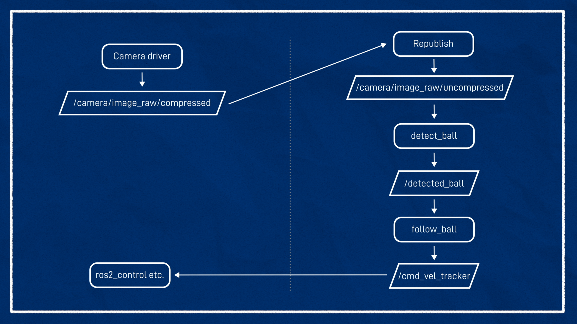
When we run all this on the robot, we don’t need to worry about any of this, as it can use the raw image with local access.
So on the dev machine we’ll run:
ros2 run image_transport republish compressed raw --ros-args -r in/compressed:=/camera/image_raw/compressed -r out:=/camera/image_raw/uncompressed
To republish the image, and we can run ball_tracker using our preferred method, as long as we remap the topic. As an example:
ros2 launch ball_tracker ball_tracker.launch.py params_file:=path/to/params.yaml image_topic:=/camera/image_raw cmd_vel_topic:=/cmd_vel_tracker enable_3d_tracker:=true
Add a new params file
We’ll duplicate our params file (ball_tracker_params_sim.yaml) and change the name to ball_tracker_params_robot.yaml. We can leave the values the same to begin with.
1
Launch and Tune
Just like before we want to:
- Launch with detections only (use the
detect_onlylaunch argument) - Have tuning mode on (use
tune_detectionlaunch argument ortuning_modenode argument if running directly) - Monitor
/image_tuningwith RViz or similar - Move the ball around in front of the camera in the environment the robot will be operating in
- Adjust the tuning until the ball is isolated
- Update the new params file with the new values
Before the next step, remember to prop the robot up so it doesn't run away!
Then we can relaunch without the detect_only and tune_detection arguments. We want to move the ball in front of the robot to check the motors are responding correctly, and if so we can let it go!
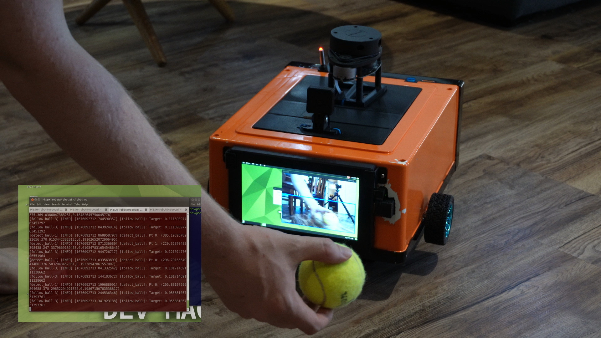
Of course if there are detection troubles, we can always go back and retune it.
Run on robot
Once we’re happy with the tuning we can push everything up to git and pull it back down on the robot. Remember to also clone the ball_tracker repo to the robot workspace, and install OpenCV.
We can then run our launch command via SSH (remember to pass the correct params file, or if using the provided example launch include, to have sim_mode off). It may be helpful to monitor /image_out either via RViz on the dev machine, or the on-screen display (remember to prefix with DISPLAY=:0 over SSH).
The robot should then follow the ball around!
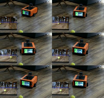
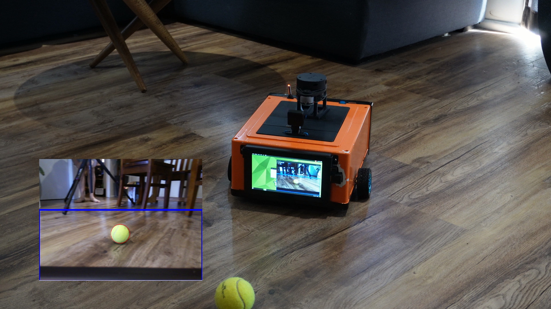
Conclusion and Improvements
This is obviously a very basic object tracking system and there are many ways we could improve it.
Some ideas are:
- More advanced object detection (e.g. faces, animals) - This could even use Neural Networks instead of classical methods.
- Depth camera - gives more information that can be used to improve both the detection and the following
- Dedicated image processing - Some chips such as the one in the OAK-D Lite can actually perform image processing onboard the camera or on another dedicated board. This is great as it takes the load off the main robot processor. It can be difficult to set up, but some systemd (such as the OAK-D) come with examples.
So now our robot can:
- Be driven remotely
- Scan a room and navigate it autonomously
- Autonomously chase an object it sees
We’re starting to get pretty close to the end of this project for now and hopefully it can serve as the basis for more projects in the future.
In the next tutorial we'll tidy up a bunch of things both in code and in hardware, then after that we’ll upgrade everything to humble.