Translations

The translation problem

So far in this series we've learnt how to use linear transformation matrices to rotate points around the origin. This is all well and good but it's really not enough to just be able to rotate points, we would also like to translate them. We need to be able to move them around the plane (left/right/up/down etc.) - otherwise we would be stuck designing robots that just spin around on the spot!

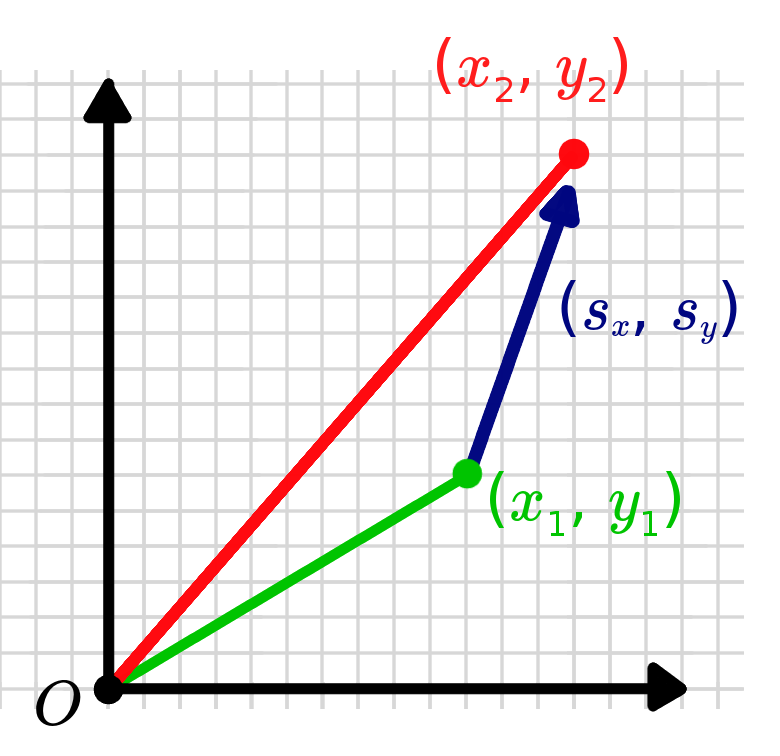
On the surface, this seems like a very straightforward problem to solve - we simply need to add the appropriate amount to the $x$ and $y$ coordinates. Say, for example, that we had the point $(x,y)$ and we wanted to shift it by $s_x$ units in the x direction and $s_y$ units in the y direction. We simply perform the following addition:

$$\begin{bmatrix} x \\ y \end{bmatrix} + \begin{bmatrix} s_x \\ s_y \end{bmatrix} = \begin{bmatrix} x + s_x \\ y + s_y \end{bmatrix}$$

Seems simple enough, right? The problem is that this operation is non-linear. If you remember, all the transformations we've looked at so far have been of the form $f(\mathbf{p}) = \mathbf{A}\mathbf{p}$ which is linear. But our translation looks like $f(\mathbf{p}) = \mathbf{p} + \mathbf{b}$.

While it's not the end of the world, having to introduce this nonlinearity is a bit unfortunate. We suddenly lose all those key properties we had with linear transformations, most notably how easily we could chain different transformations together. You'll recall that if we had three nested transformations we could simply multiply the matrices together: $f_3(f_2(f_1(\mathbf{p}))) = \mathbf{A}_3\mathbf{A}_2\mathbf{A}_1\mathbf{p}$.

Let's take a look at what happens if we want to perform the following steps:

1. Shift a point by $(s_x, s_y)$, then
2. Rotate it by $\theta$, then
3. Shift it again by $(t_x, t_y)$, then
4. Rotate it by $\phi$

This chain produces the following equation:

$$\begin{align*}\mathbf{p}_2 &= \mathbf{R}(\phi)(\mathbf{R}(\theta)\mathbf{p} + \mathbf{s}) + \mathbf{t} \\ &= \mathbf{R}(\phi) \mathbf{R}(\theta)\mathbf{p} + \mathbf{R}(\phi)\mathbf{s} + \mathbf{t}\end{align*}$$

If we were to write these matrices out in full, the equation quickly becomes very confusing. On top of that, inverting the combined transformation becomes really awful. There must be a better way! Thankfully, there is.

Introducing... Homogeneous Coordinates!

To solve this problem we're going to introduce a slightly modified representation of our coordinates. This new system is called homogeneous coordinates. What we'll discover in this post and the next is that by using a homogeneous coordinate system, we can represent both rotations and translations using a single matrix. In this post, we'll focus solely on the translation.

The first thing we have to do is modify our coordinates, which simply involes tacking a "$1$" onto the end of our point vector. For the next little while we will use the bar ($\bar{\phantom{p}}$) above our various variable names to express that they are working with the homogeneous coordinates, but in later posts it will just be assumed.

$$\bar{\mathbf{p}} = \begin{bmatrix} x \\ y \\ 1 \end{bmatrix}$$

Deriving the Translation Matrix

What we want to try to do now is to find a linear transformation in this new coordinate system that would represent our translation. In 2D, this will mean we are looking for a $3 \times 3$ matrix to multiply by $\bar{\mathbf{p}}$ that is equivalent to adding $\mathbf{s} = [s_x, s_y, 0]^\text{T}$.

$$\bar{\mathbf{p}}_2 = \mathbf{A} \bar{\mathbf{p}}_1 = \bar{\mathbf{p}}_1 + \mathbf{s}\\ \begin{bmatrix} x_2 \\ y_2 \\ 1 \end{bmatrix} = \begin{bmatrix} ? & ? & ? \\ ? & ? & ? \\ ? & ? & ? \end{bmatrix}\begin{bmatrix} x_1 \\ y_1 \\ 1 \end{bmatrix} = \begin{bmatrix} x_1 + s_x\\ y_1 + s_y \\ 1 \end{bmatrix}$$

Let's figure this out, step by step. Firstly, we need to guarantee a $1$ in the bottom element of the result. To achieve this, the elements in the bottom row of our matrix will need to be all $0$, except for a $1$ at the end.

$$\begin{bmatrix} ? & ? & ? \\ ? & ? & ? \\ 0 & 0 & 1\end{bmatrix}\begin{bmatrix} x_1 \\ y_1 \\ 1 \end{bmatrix} = \begin{bmatrix} ? \\ ? \\ 1 \end{bmatrix}$$

Secondly, we know that for the first element of our result, there is one $x_1$ and no $y_1$, and vice versa for the second element. To get this, we put a little identity matrix in the top left corner.

$$\begin{bmatrix} 1 & 0 & ? \\ 0 & 1 & ? \\ 0 & 0 & 1\end{bmatrix}\begin{bmatrix} x_1 \\ y_1 \\ 1 \end{bmatrix} = \begin{bmatrix} x_1 + ? \\ y_1 + ? \\ 1 \end{bmatrix}$$

Lastly, the top of the right column of our matrix will contain the column vector we want to translate by.

$$\begin{bmatrix} 1 & 0 & s_x \\ 0 & 1 & s_y \\ 0 & 0 & 1\end{bmatrix}\begin{bmatrix} x_1 \\ y_1 \\ 1 \end{bmatrix} = \begin{bmatrix} x_1 + s_x \\ y_1 + s_y \\ 1 \end{bmatrix}$$

And we're done! By using homogeneous coordinates, we can represent our non-linear translation as a linear transformation. The reason this works is that although a translation is not a linear transformation, it falls under a bigger subset of non-linear transformations called affine transformations. This will work in 2D, 3D, or however many dimensions you want!

Examples

Geogebra

Loading

MATLAB/Octave

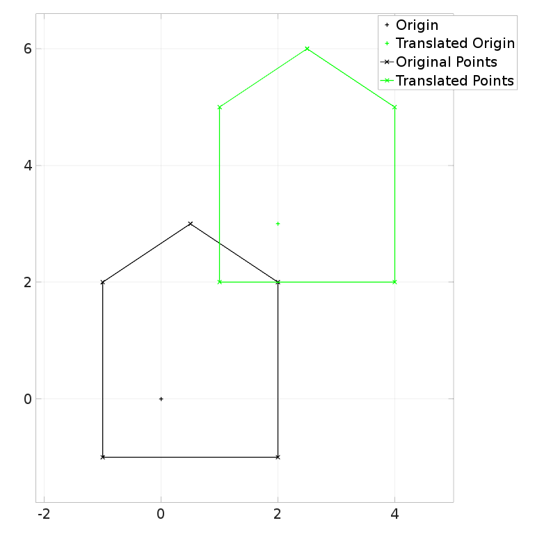
% Set up an array of points
x_points = [2, 2, 0.5, -1, -1, 2];
y_points = [-1, 2, 3,  2, -1, -1];
points = [x_points; y_points; ones(1, length(x_points))];
    
% Translation matrix
sx = 2; sy = 3;
trans_mat = [1, 0, sx; ...
             0, 1, sy; ...
             0, 0,  1];                                
             
% Transform the points
for p = 1:size(points,2)
  trans_pts(:,p) = trans_mat * points(:,p);
end            

% Plot everything
clf;
plot(0,0,'+k', 'DisplayName', 'Origin');
hold on;
plot(sx,sy,'+g', 'DisplayName', 'Translated Origin');
plot(points(1,:), points(2,:), 'x-k', 'DisplayName', 'Original Points');
plot(trans_pts(1,:), trans_pts(2,:), 'x-g', 'DisplayName', 'Translated Points');
legend show; grid on; axis equal;