Linear vs. Nonlinear Transformations
In the last post we started to explore how we can use coordinate transformations to manipulate points in space, and set ourselves the task of finding the transformations that would let us represent a robot that moves and rotates around in its environment.
An important step in this is to understand that we can separate all transformations into two distinct categories: linear and non-linear. We'll talk in more detail about what linearity means later, but for now all we need to know is that for our purposes 1 linear functions are functions of the form:
Where is an matrix, and is the number of dimensions in . So the matrix for the 1D, 2D, and 3D cases respectively would look like:
If the function is anything other than a matrix multiplied by the input then it is non-linear. And while this seems like a pretty heavy limitation (as we'll see in future posts) we can still do some impressive transformations, and understanding how to use them will set us up well for understanding non-linearities further down the track.
Just a quick warning, don't be fooled into thinking a function like is linear just because it is a line. Being linear in the polynomial sense is not the same as being a linear function/transformation, and that particular function is non-linear due to the added term.
Exploring Linear Transformations
Let's explore this idea a bit further using the example of a 2D linear transformation. We'll have a look at how each of these four matrix elements (, , , and ) will influence the behaviour of our transformation.
The Identity Matrix
The first, and simplest matrix we will look at is the identity matrix (i.e. and are , and are ). When we multiply any vector by the identity matrix, we get the same vector out - so this transformation does nothing! This will be our starting point for looking at the other transformations.
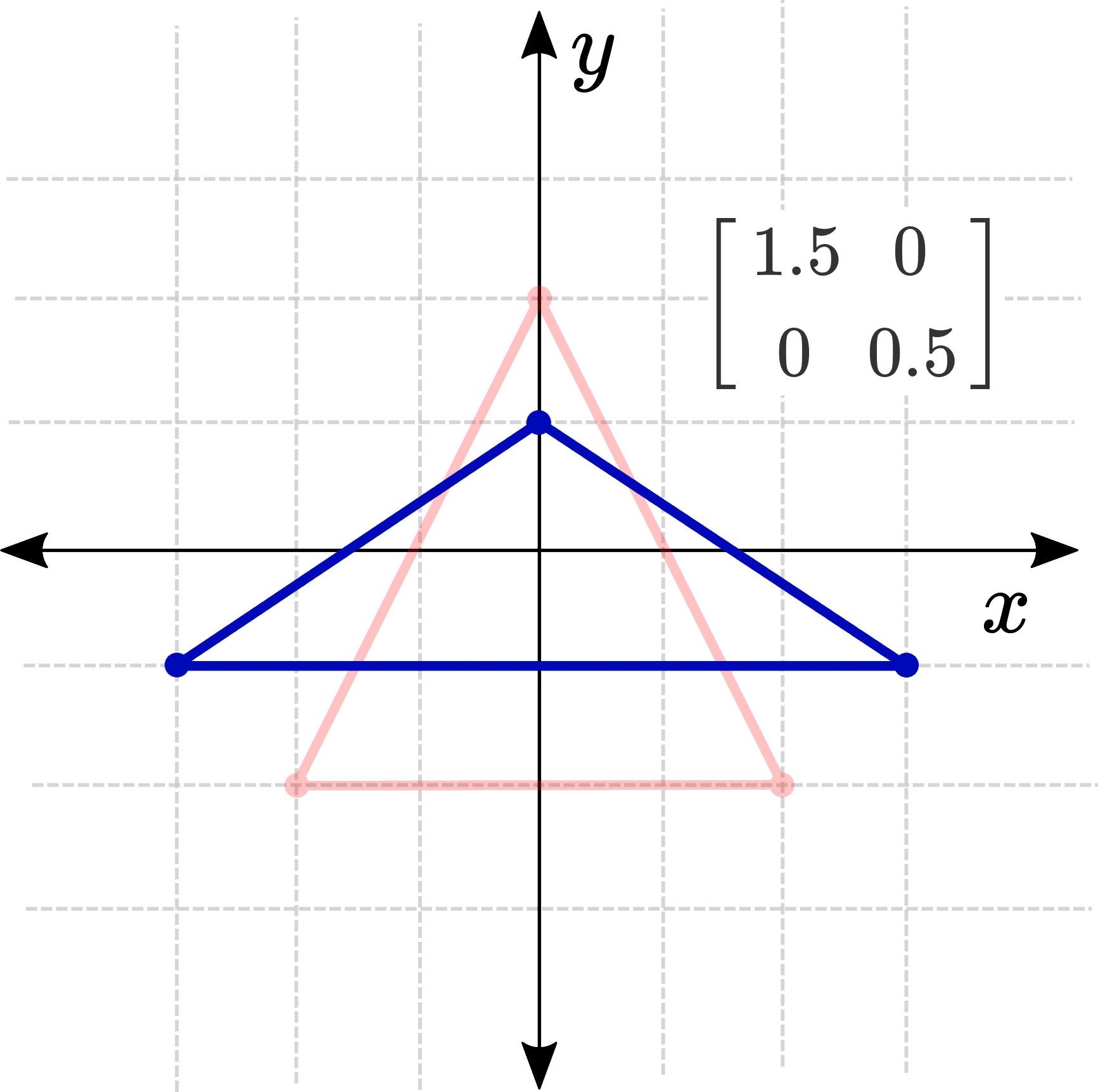
Scaling
The element will determine how much affects , and the element will determine how much affects . If we only change these values, this will result in a scale in the or axis (or both). Reducing both of these to zero is a special case where every single point is shrunk down into the origin!
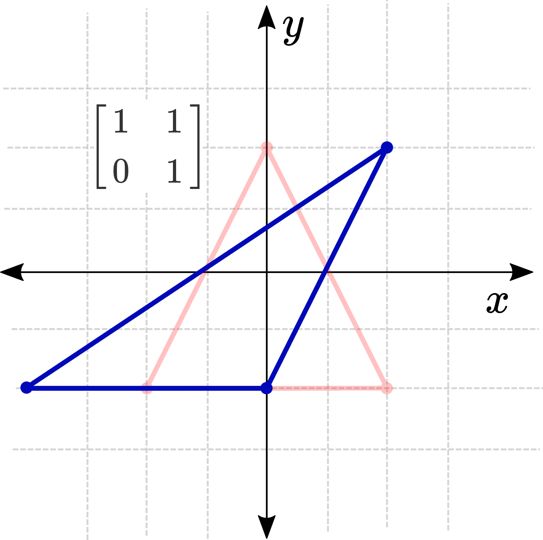
Shearing
The two off-diagonal elements control the shear transform. The element determines how much the old affects the new , and the element determines how much the old affects the new . Keeping and at 1 and adjusting these one at a time produces a shear/skew effect.
Combinations
Combining these lets us produce some other interesting effects. For example, if we use the matrix we are saying that the new is only influenced by the old and vice versa. This results in a mirror of all the points across the line .
Have a play around with the Geogebra example at the bottom of the page and see if you can find a combination that will rotate all the points around the origin by 90 degrees.
Properties of linear transformations
So why do we care so much about linear transformations? Well all linear transformation have a bunch of useful common properties that make them much more pleasant to work with, compared to non-linear functions. Here are a few:
- always maps to . There is no way to move the origin.
- Linear transformations are always odd (). This results in a sort of mirroring effect. If you pick any point and see how it moves, the point exactly opposite (through the origin) will move the opposite way, and will continue to be its mirror. You can imagine there is a pin through the origin and everything is stretching and mirroring around it.
- Linear transformations chain through multiplication. If we want to scale some points, then shear them, then rotate them, we just need to multiply all the matrices together:
This last property is extremely helpful. It doesn't just make the equations simpler on page, it also improves computation speed as we can pre-multiply the matrices as necessary, and then transform whatever points we need with a single final multiplication.
Conclusion
It might seem like we've strayed a little from our task - we were looking for practical transformations, ones that translate and rotate our points. However, even though real robots don't scale or shear, understanding the structure of linear transformations is important because if we can find a way to translate and rotate within this framework it will make our calculations far simpler.
Examples
Geogebra
Start by adjusting the sliders one at a time, returning them to their start values after each adjustment. Try doing two or more at a time to see what effects it causes. Can you create a rotation? What about a translation?
Loading
MATLAB/Octave
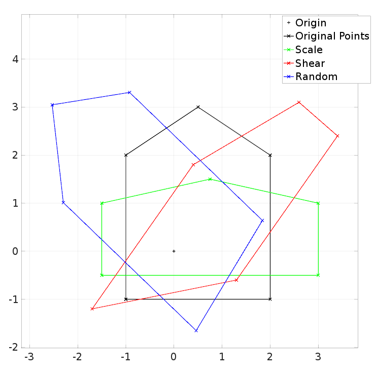
The MATLAB script below generates a small "house" shape, offset from the origin. It then shows what the house would look like with the following transformations:
- A scale change (both X and Y)
- A shear (both X and Y)
- A randomly generated transformation (note that if you run the code you'll get a different shape for this one)
Try changing the numbers for one of them and see what you get!
% Set up an array of points
x_points = [2, 2, 0.5, -1, -1, 2];
y_points = [-1, 2, 3,  2, -1, -1];
points = [x_points; y_points;];

% Scale
scale_mat = [1.5,   0; ...
               0, 0.5];

% Shear
shear_mat = [  1, 0.7; ...
             0.2, 1];

% Random
rand_mat = 3*rand(2) - 1.5;

% Transform the points
for p = 1:size(points,2)
  scale_pts(:,p) = scale_mat * points(:,p);
  shear_pts(:,p) = shear_mat * points(:,p);
  rand_pts(:,p) = rand_mat * points(:,p);
end

% Plot everything
clf;
plot(0,0,'+k', 'DisplayName', 'Origin');
hold on;
plot(points(1,:), points(2,:), 'x-k', 'DisplayName', 'Original Points');
plot(scale_pts(1,:), scale_pts(2,:), 'x-g', 'DisplayName', 'Scale');
plot(shear_pts(1,:), shear_pts(2,:), 'x-r', 'DisplayName', 'Shear');
plot(rand_pts(1,:), rand_pts(2,:), 'x-b', 'DisplayName', 'Random');
legend show; grid on; axis equal;
Extra Resources
- Wikipedia has an article on the broader mathematical definition of linear functions/maps/transformations (of which we are looking at a subset - coordinate transformations).
Footnotes
-
We are assuming that the problem to solve is a single-input, single-output problem where the input space and output space are of the same dimension. ↩