2D Rotations

In the last post we saw that we can use matrices to perform various kinds of transformations to points in space. We can stretch, flip, and scale them, but the important one for us is rotation. Robots don't suddenly scale their size up and down, and they certainly don't mirror themselves along an axis, but one thing they do quite frequently is rotate. Because of this, it's important that we have a solid mathematical understanding of the rotation of points in space.

Deriving the rotation matrix

Say we have a point $(x_1, y_1)$ and we want to find the $2\times2$ transformation matrix that will rotate it (anticlockwise) around the origin by an angle $\theta$ to a new point, $(x_2, y_2)$.

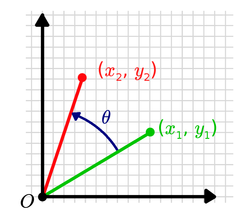
In other words, we're looking for values to satisfy an equation that looks something like this:

$$\begin{bmatrix} x_2 \\ y_2 \end{bmatrix} = \begin{bmatrix} a & b \\ c & d \end{bmatrix} \begin{bmatrix} x_1 \\ y_1 \end{bmatrix} = \begin{bmatrix} a x_1 + b y_1 \\ c x_1 + d y_1 \end{bmatrix}$$

To tackle this, we'll start by adding some extra variables to make life easier. We'll add $h$, the distance from the point to the origin (the hypotenuse of the triangle formed by $(0,0)$, $(x_1, 0)$, and $(0, y_1)$), and $\phi$, the angle the hypotenuse makes with the x-axis.

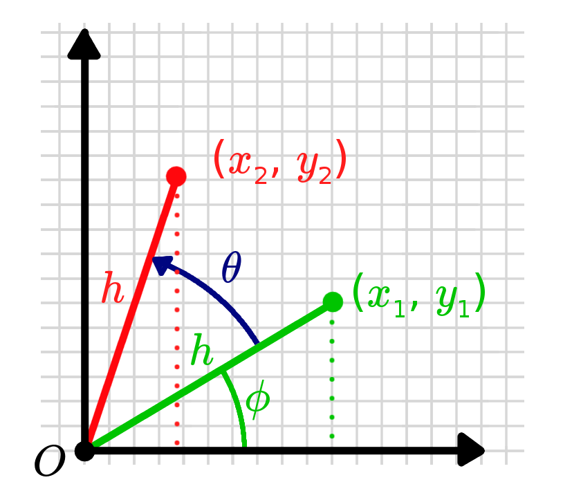
We can now express $x_1$ and $y_1$ in the following way:

$$\begin{bmatrix} x_1 \\ y_1 \end{bmatrix} = \begin{bmatrix} h\cos(\phi) \\ h\sin(\phi) \end{bmatrix}$$

We can express the new, rotated point similarly. It should be at the same distance from the origin, $h$, but at a new angle, $(\phi + \theta)$. Then, by using some trig identities, we can substitute our original points back in.

$$\begin{align*}\begin{bmatrix} x_2 \\ y_2 \end{bmatrix} &= \begin{bmatrix} h\cos(\phi + \theta) \\ h\sin(\phi + \theta) \end{bmatrix} \\ &= \begin{bmatrix} h\cos(\phi)\cos(\theta) - h\sin(\phi)\sin(\theta) \\ h\sin(\phi)\cos(\theta) + h\cos(\phi)\sin(\theta) \end{bmatrix} \\ &= \begin{bmatrix} x_1\cos(\theta) - y_1\sin(\theta) \\ x_1\sin(\theta) + y_1\cos(\theta) \end{bmatrix}\end{align*}$$

We can now pull out the coefficients and express this as a matrix multiplied by the first point:

$$\begin{bmatrix} x_2 \\ y_2 \end{bmatrix} = \begin{bmatrix} \cos(\theta) & -\sin(\theta) \\ \sin(\theta) & \cos(\theta) \end{bmatrix}\begin{bmatrix} x_1 \\ y_1 \end{bmatrix}$$

And that's it! That $2 \times 2$ matrix is the 2D rotation matrix. You can multiply it by any point (or series of points) to rotate them anticlockwise about the origin by the angle $\theta$. If you'd like to see some examples, you can scroll to the bottom of the page. But first, we'll take a closer look at three important properties that a rotation matrix has.

Properties of rotation matrices

Rotation matrices have a few important properties that make them really useful. They might seem a bit trivial to begin with, but as we work with more complex equations and many matrices, they will save a lot of headaches!

Inverse = Transpose

The first property to be aware of is that the inverse of a rotation matrix is its transpose. Sometimes computing the inverse of a matrix can be quite a difficult (or even impossible) task, but with a rotation matrices it becomes very straightforward.

There's actually a pretty simple way to understand this relationship. Imagine that we have a point $(x_2, y_2)$ that we got by rotating a point $(x_1, y_1)$ by an angle $\theta$. If we want to invert this transformation, that is the same as "un-rotating" the point, or equivalently to rotate it by an angle $-\theta$.

$$\begin{align*}R(\theta)^{-1} &= \begin{bmatrix} \cos(\theta) & -\sin(\theta) \\ \sin(\theta) & \cos(\theta) \end{bmatrix}^{-1} \\ &= \begin{bmatrix} \cos(-\theta) & -\sin(-\theta) \\ \sin(-\theta) & \cos(-\theta) \end{bmatrix}\end{align*}$$

Using the fact that cosine function is even ($\cos(-\theta) = \cos(\theta)$) and the sine function is odd ($\sin(-\theta) = -\sin(\theta)$), the result can be proved quite easily.

$$\begin{align*}R(\theta)^{-1} &= \begin{bmatrix} \cos(-\theta) & -\sin(-\theta) \\ \sin(-\theta) & \cos(-\theta) \end{bmatrix} \\ &= \begin{bmatrix} \cos(\theta) & \sin(\theta) \\ -\sin(\theta) & \cos(\theta) \end{bmatrix} \\ &= \begin{bmatrix} \cos(\theta) & -\sin(\theta) \\ \sin(\theta) & \cos(\theta) \end{bmatrix}^{T} \\ &= R(\theta)^{T} \end{align*}$$

Determinant = 1

The second property is that the determinant of all rotation matrices is equal to one, no matter what the value of $\theta$ is. Again, this is pretty straightforward to prove using the equation for the determinant of a 2D matrix and some standard trig identities.

$$\det \left(\begin{bmatrix} a & b \\ c & d \end{bmatrix}\right) = ad-bc$$

x

$$\begin{align*} \det(R(\theta)) &= \det \left(\begin{bmatrix} \cos(\theta) & -\sin(\theta) \\ \sin(\theta) & \cos(\theta) \end{bmatrix}\right) \\ &= (\cos(\theta)\cos(\theta)) - (-\sin(\theta)\sin(\theta)) \\ &= \cos^2(\theta) + \sin^2(\theta) \\ &= 1\end{align*}$$

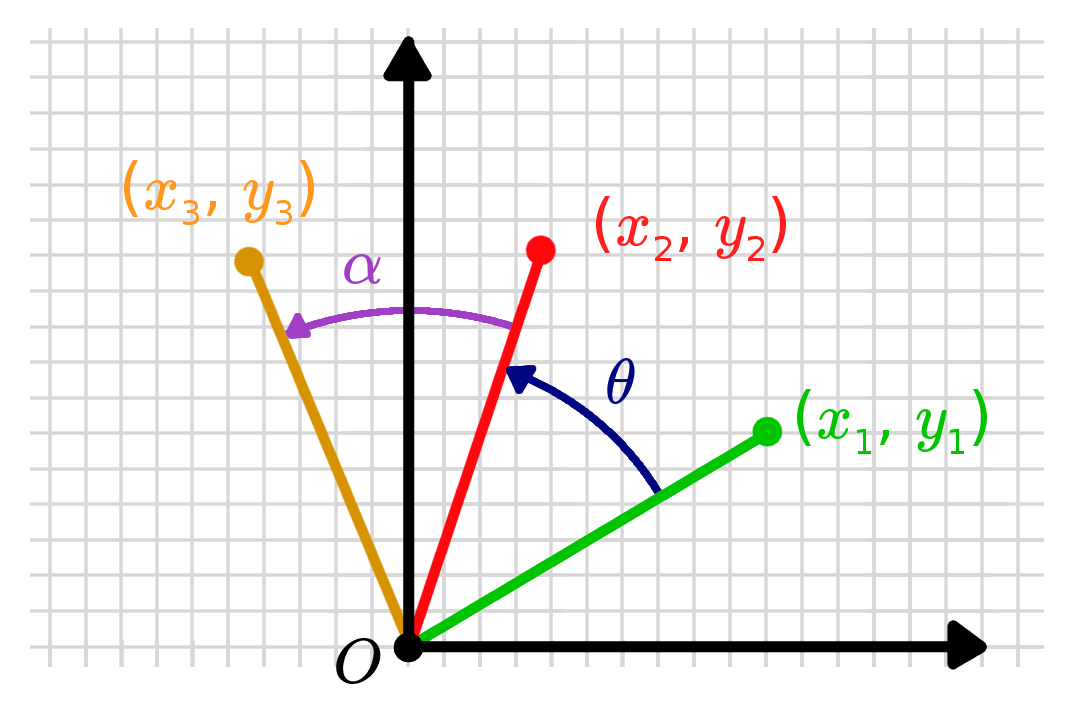
Rotation X Rotation = Rotation

Rotation matrices have the property that if you multiple two of them together, you always get another rotation matrix. That is, you get another matrix that has the same properties as above and which would represent a different rotation in space (for the 2D case it will be the sum of the two angles of the original, but in 3D it will get more interesting).

Again, we can prove this fairly easily with trig identities.

$$\begin{align*}R(\alpha) R(\theta) &= \begin{bmatrix} \cos(\alpha) & -\sin(\alpha) \\ \sin(\alpha) & \cos(\alpha) \end{bmatrix} \times \begin{bmatrix} \cos(\theta) & -\sin(\theta) \\ \sin(\theta) & \cos(\theta) \end{bmatrix} \\ &= \begin{bmatrix} \cos(\alpha)\cos(\theta) - \sin(\alpha)\sin(\theta) & -\cos(\alpha)\sin(\theta) - \cos(\alpha)\sin(\theta) \\ \sin(\alpha)\cos(\theta) + \cos(\alpha)\sin(\theta) & -\sin(\alpha)\sin(\theta) + \cos(\alpha)\cos(\theta) \end{bmatrix} \\ &= \begin{bmatrix} \cos(\alpha + \theta) & -\sin(\alpha + \theta) \\ \sin(\alpha + \theta) & \cos(\alpha + \theta) \end{bmatrix} \\ &= R(\alpha + \theta)\end{align*}$$

Other Properties (and other names!)

Rotation matrices also have some other properties that we won't explore here. One thing worth noting is that the fancy mathematical name for the group of all rotation matrices is the "special orthogonal group" (for a particular dimension $n$). You might sometimes see it written that a matrix is in $SO(2)$ or $SO(3)$ - this simply means it is a rotation matrix in 2D or 3D respectively.

Where to next?

Now that we have the mathematics of 2D rotations down pat, there are two burning questions on the table. Firstly, how can we express a translation (an overall position shift) in this same form? And secondly, how do we extend this knowledge into 3D? A robot that simply sits on the ground and spins around in a circle isn't very interesting - in reality, most useful robots move around. For something like a multirotor or a submarine, it will be constantly translating and rotating in all three dimensions.

Over the next three posts we will explore how to use a similar language to express translations, combined rotations and translations, and then how to apply it all in 3D.

Examples

Geogebra

Loading

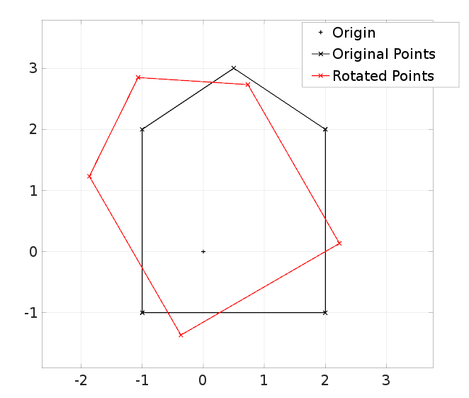
MATLAB/Octave

% Set up an array of points
x_points = [2, 2, 0.5, -1, -1, 2];
y_points = [-1, 2, 3,  2, -1, -1];
points = [x_points; y_points];

% Rotation matrix
theta = 30;
rot_mat = [cosd(theta), -sind(theta);
           sind(theta),  cosd(theta)];

% Rotate the points
for p = 1:size(points,2)
  rot_pts(:,p) = rot_mat * points(:,p);
end            

% Plots
clf;
plot(0,0,'+k', 'DisplayName', 'Origin');
hold on; grid on;
plot(points(1,:), points(2,:), 'x-k', 'DisplayName', 'Original Points');
plot(rot_pts(1,:), rot_pts(2,:), 'x-r', 'DisplayName', 'Rotated Points');
legend show; axis equal;

Extra Resources

• Wikipedia has an article covering some of the features of both 2D and 3D rotation matrices.