Introducing Coordinate Transforms
Why do we care about coordinate transformations?
A huge part of robotics (and engineering in general) is representing different aspects of the physical world mathematically. This is necessary so that we can then design control systems, plan trajectories, predict future motion, etc. There are many different ways we can represent the robots and their environment depending on the problem to be solved. For example, someone designing a control system will be very interested in the different forces at play, the sensors and actuators that are available, and will be trying to model the "physics" of the system.
In these posts we're not interested in that at all. This is about developing a robust mathematical "language" to describe the overall shape of a robot as it moves through space. The immediately obvious applications for this are in simulation and visualisation - this will let us take the information about positions and rotations that come from a dynamic model and show what it would actually look like - but eventually we will see how this can feed back into the model and give us a cleaner structure for processing sensors and controlling actuators. Having a solid understanding in this area can take a problem that seems ridiculously complex and fiddly and reduce it to a couple of lines.
Throughout this series we will be looking at robots as a series of points in space (coordinates) and how we can manipulate (transform) those points appropriately, given the positions and orientations.
Representing a robot as points in space
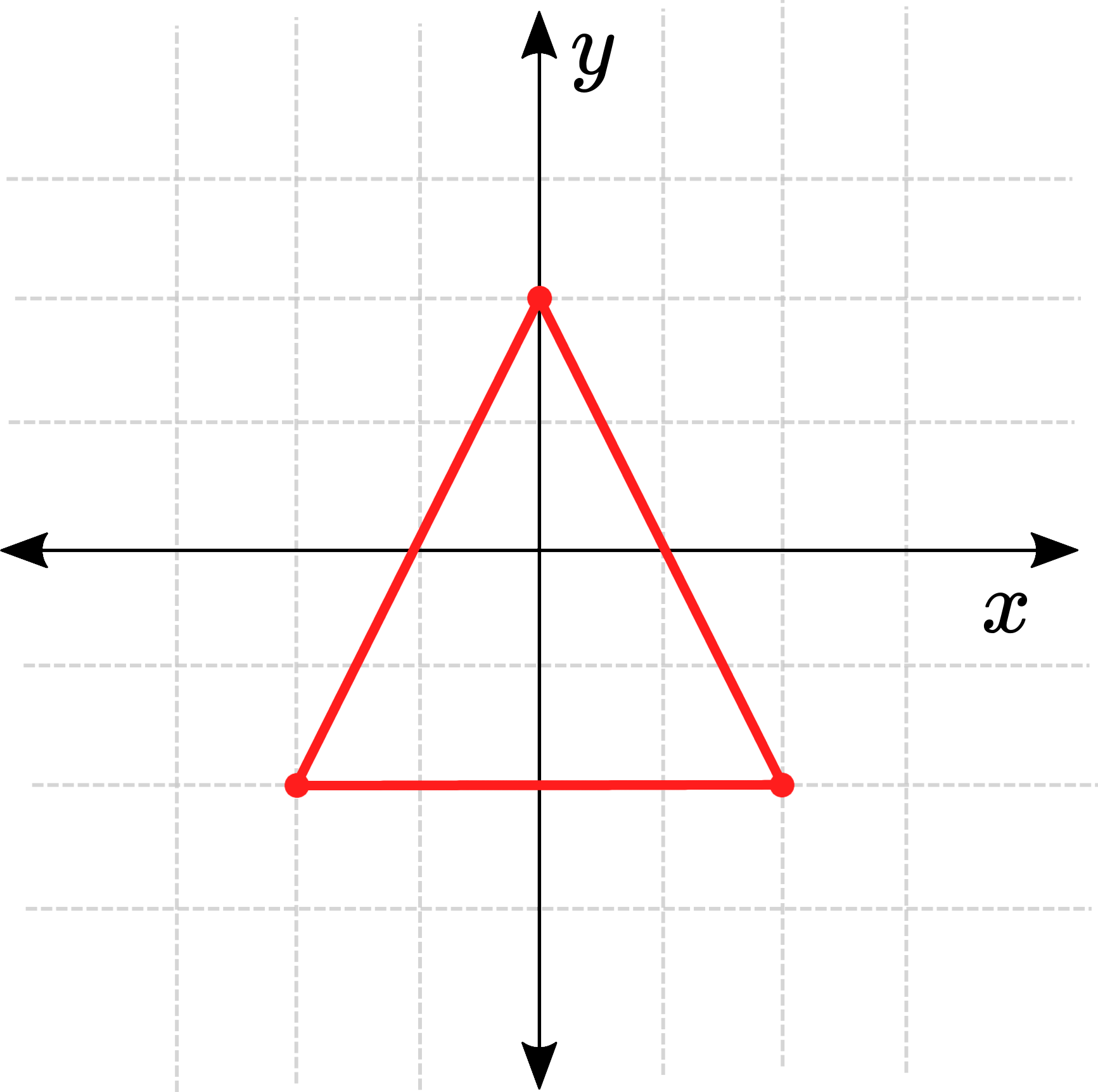
The very first step in coming up with a mathematical description for our robot's motion in space, is to figure out how we will describe the robot itself. The simplest way to do this is with a single point:
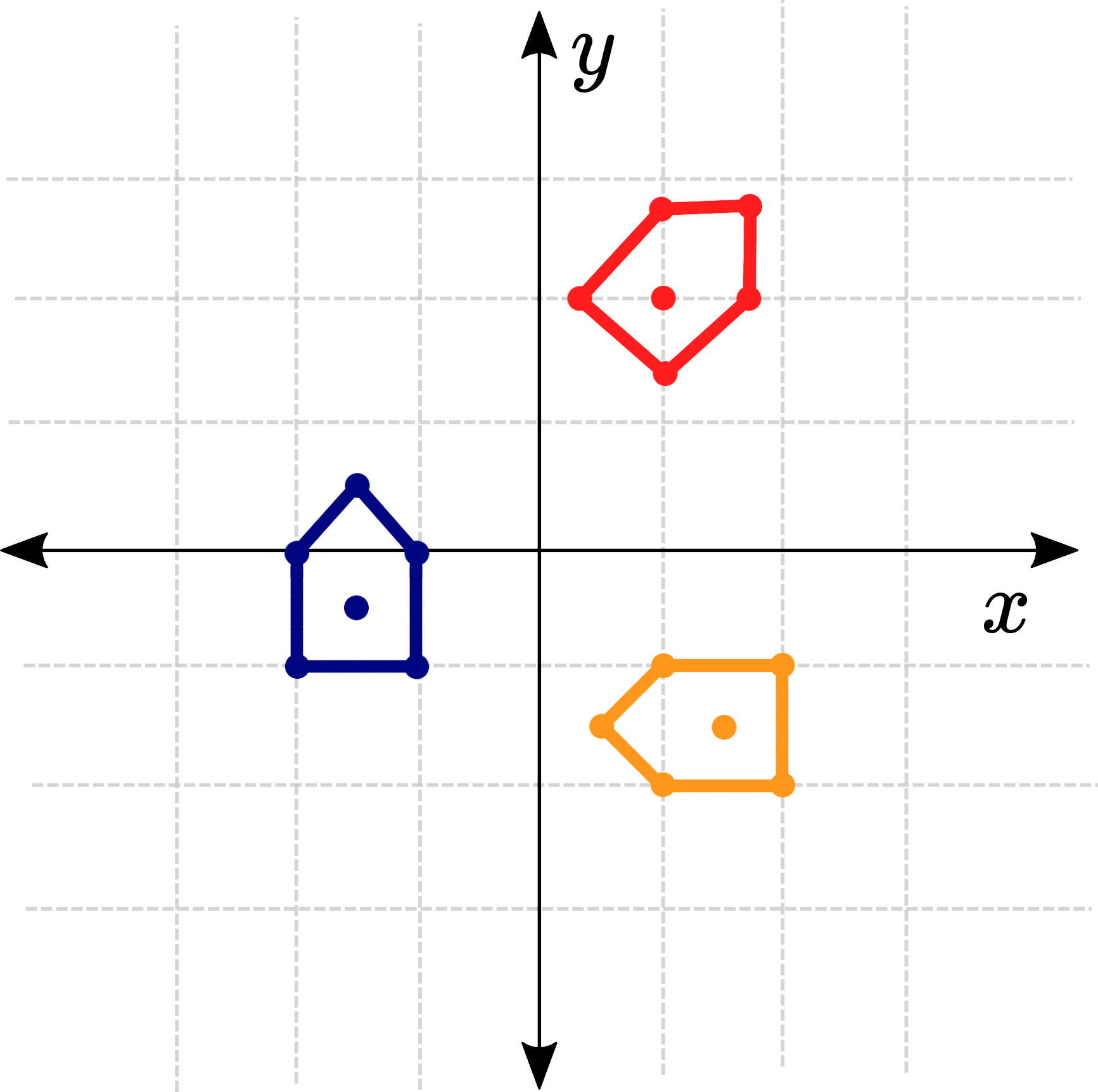
We could move this point around in space and it would show where the robot moves, but it just seems a bit...lacking. For one, it doesn't have any way to show the rotation of our robot. It also doesn't give any shape or scale to our robot, we can't tell how big it is. To fix this, we can use a series of points instead. This could be simple, such as a rectangle or triangle, or a complex CAD model - depending on the requirements. Now, if we place the robot at different positions and orientations we can get really get a sense of how it moves about in space.
For many robots, movement is restricted to a single plane (e.g. the ground or the surface of water) and a 2D representation is sufficient - and much easier to calculate. For systems that move around in full 3D such as a multirotor, a 3D representation will be necessary.
In the beginning of this series, we will be learning how to describe robots in this way, as a simple set of points moving around in space. After that we will extend our approach by introducing the concept of multiple coordinate systems and reference frames, which helps to simplify some of the mathematics when dealing with more complex systems.
Throughout all these posts, a point is generally represented as a column vector with two or three elements (, , and ) depending on whether it is in 2D or 3D 1. While there are situations where alternative systems such as polar coordinates may be more appropriate, for the vast majority of applications a cartesian system like this will be most useful.
Now that we have a way to represent our robot in space mathematically, we're going to explore how we can manipulate these points and make our robot move.
Transforming points with a function
1D Functions
Most of us are probably familiar with the idea of a function from maths. A function takes an input, or a series of inputs, and maps them to a single output. We're mostly used to functions that work in one dimension. They take the form or something like that, where each variable is a scalar (one dimension).
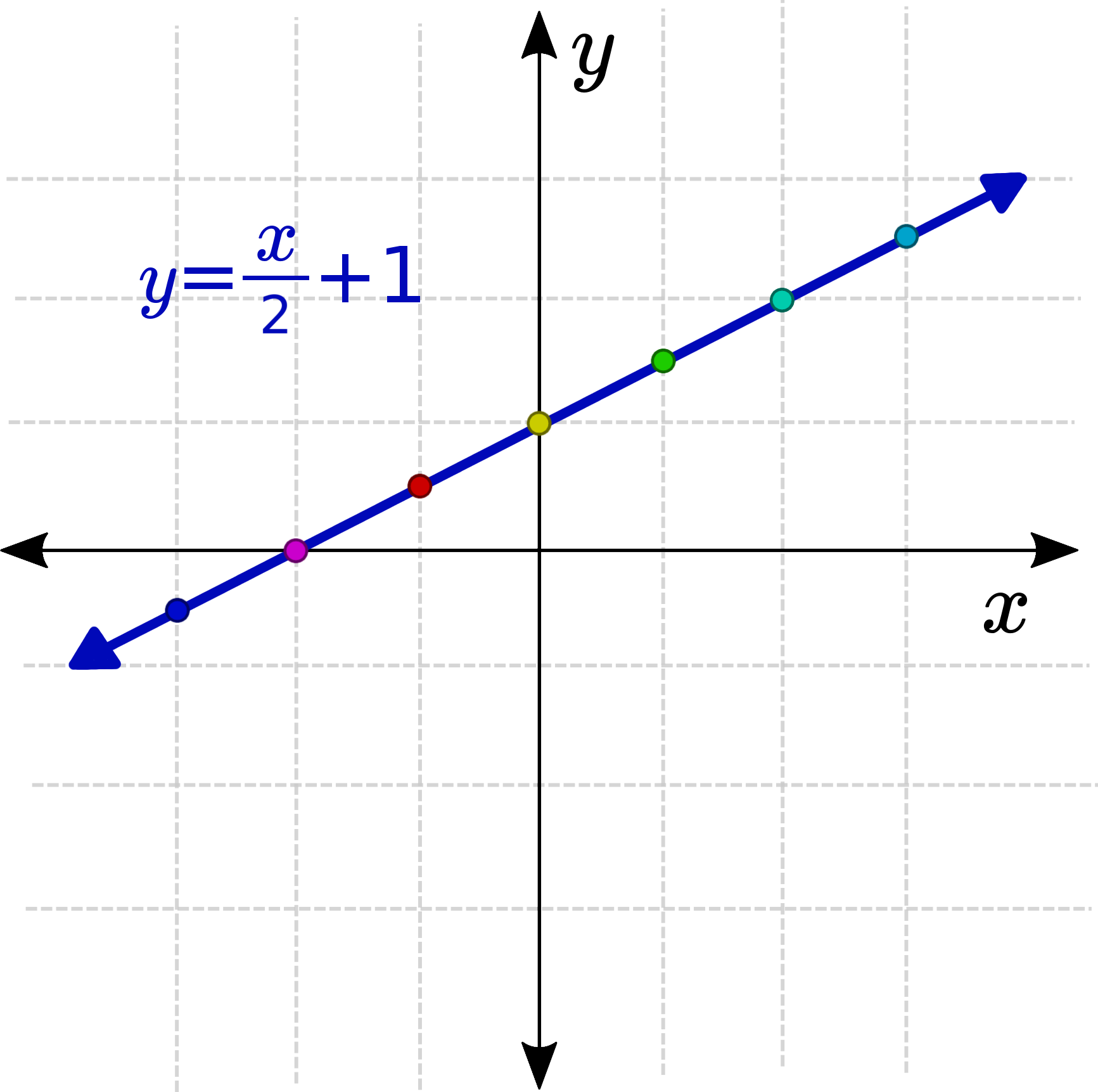
A simple example might be , or . This function takes the values and transforms them, or maps them to new values. Any value you pick will have a corresponding value. Typically, we choose to represent this using a 2D plane where we have the horizontal axis representing the input value , and the vertical axis representing the output value . So a single 1D input maps to a single 1D output , represented in 2D.
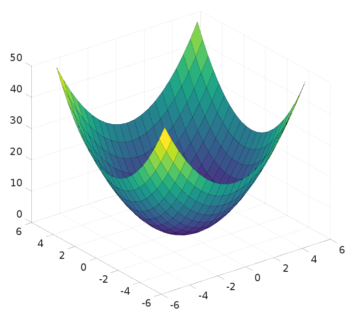
The next step from there is functions of multiple inputs. You might have the function for a 3D parabola, . This function takes two 1D inputs ( and ), and maps them to a single 1D output (), so we use three dimensions to represent it. Keep in mind that this is still a 1D problem!
1D Functions - An alternative view
Before we move on though, let's think about a different way to represent the first (single-input, single-output) case, . Rather than plotting it in the 2D plane like we did before, we can instead plot it as two separate 1D number lines.
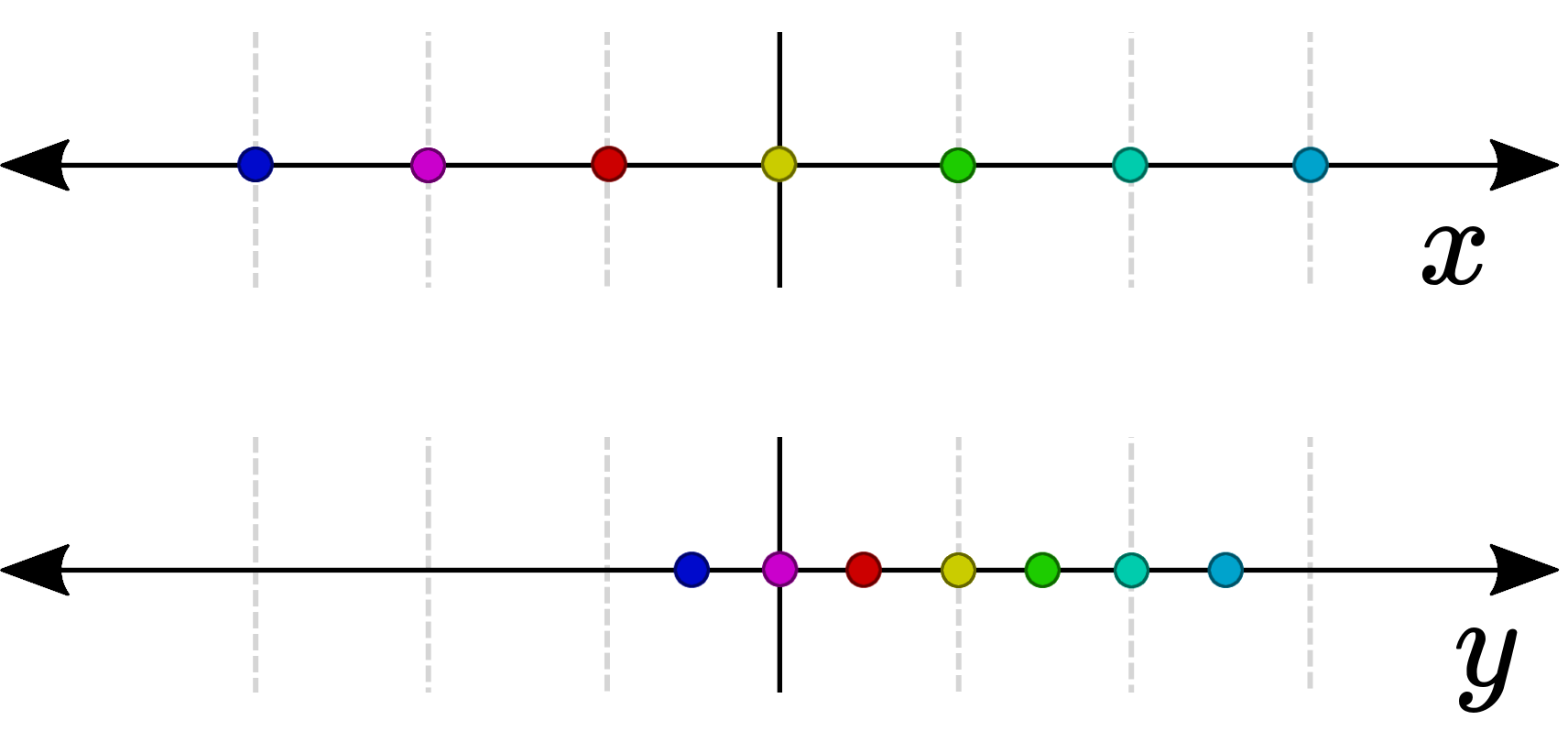
Note how each point in the input space has a corresponding point in the output space. Three example points are shown in the table below.
| Input | Output |
|---|---|
Make sure you take some time to understand the relationship between this image, and the blue line plot we saw earlier. These are two different ways of representing the same function!
2D and 3D functions
In real life our robots don't live in a 1D world. They live in a "2D" world (if they are restricted to a planar surface), or a 3D world. So if we want to use mathematics to describe the movement of our robots in space, we need to be able to use functions in higher dimensions.
Let's start with 2D. We'll write a function that takes a single 2D input and maps it to a single 2D output. Instead of using and to represent our inputs and outputs (which will quickly get confusing) let's use and 2. So our point in 2D will have an and a component:
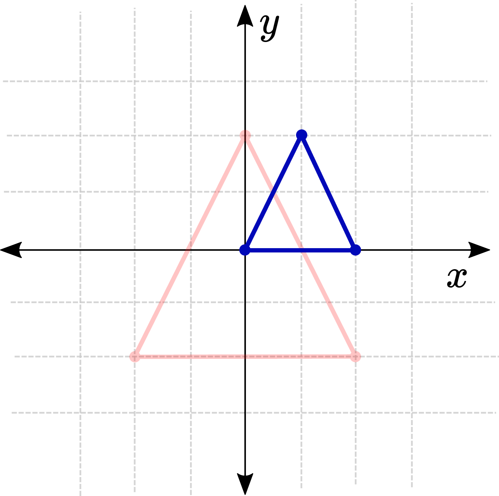
Our 2D function will look something like the equation below. It takes any point in and spits out the mapped point. Every point in 2D space (at least in our examples) can go into it, and will have some corresponding 2D output.
If we tried to represent this with a dimension for each number we would need a four-dimensional graph (which is a bit too tricky to draw), so instead we'll use the "number-line" method from before. This time, though, instead of two lines we'll have two planes since both our input space and output space are 2D. For this example, we'll use a similar function as earlier: .
Take a look at the test points in the table below and see how the function transforms them.
| Input | Output |
|---|---|
This same idea extends into 3D (and higher dimensions), we just need to add the value to our points and we can transform them through three-dimensional space.
What sort of transformations are we looking for?
While there are an infinite number of weird and wacky coordinate transformations we could come up with, in robotics there are really only two that we're interested in. As robots move through space they translate, and they rotate. Over the next few posts we're going to explore how we can use matrices to perform these coordinate transformations in both 2D and 3D. In doing so we'll develop a solid mathematical framework and language that we can use to descibe robotic motions, which will make the larger problems of robotics (control, planning, simulation, etc.) much easier.
Click here to read the next post in this series, on linear and non-linear transformations.
Footnotes
-
Later, when we introduce homogeneous coordinates, our points will sometimes be represented with an extra element which is always a . ↩
-
Don't worry too much about the exact names and notation used - everyone will do things a little differently. The important thing is to understand the structure of it all. ↩