3D Rotations

Recap

First, let's recap what we've covered so far.

We saw that using a single 2x2 matrix we can represent a whole host of transformations in the 2D plane - rotations in particular. Next, we saw that by using a 3x3 matrix and homogenous coordinates we are able to represent a translation in 2D, and in fact we can combine that with our rotation matrix to express any combination of rotation and translation in 2D using a single 3x3 matrix.

But we don't live in a flat, two-dimensional paper world, we live in a 3D space where we can rotate things in all sorts of complicated ways! So how can we take what we've learnt about transformations in 2D and apply it to 3D problems?

Extending into the third dimension

For the rest of this post we'll be exploring 3D rotation matrices, which aren't too difficult to get the hang of once you're on top of the 2D ones. However, the topic of 3D rotations in general is actually quite complicated and the maths can get a little mind-bending. Hang in there though!

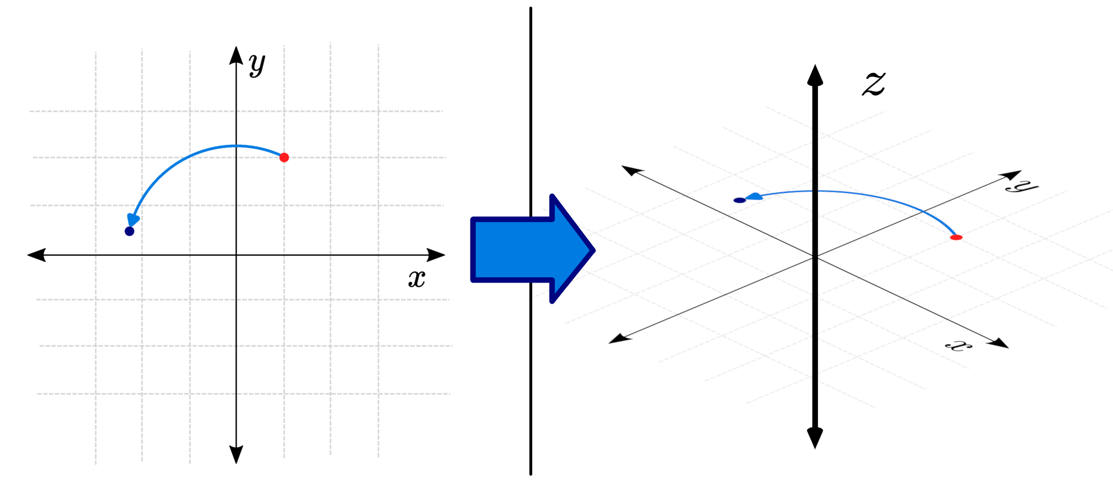
So far the rotations we have been looking at have been occurring in the X-Y plane, the normal 2D plane. The first step that we'll take in exploring 3D rotations is to simply imagine this flat plane existing within a 3D world.

When we add a third dimension, we add it in the Z direction. According to the right-hand rule, the Z direction is "out of the page" compared to the typical X-Y plane.

Suddenly, this gives us a new approach to thinking about our 2D rotations. Rather than thinking of them as just rotating points about the origin, we can think of them as rotating around the Z axis. The right-hand grip rule comes into play here. It tells us that if we look from above, a positive rotation around the Z axis is an anticlockwise rotation (i.e. moving from the positive X axis through the first quadrant to the positive Y axis). This matches what we saw in 2D, where a positive rotation was anticlockwise around the origin.

Rotating about the Z axis

With this in mind, let's think about how we can express the 2D rotations we already know. First, we're going to need to add a $z$ value to our coordinate vector to give us:

$$\begin{bmatrix}x \\ y \\ z\end{bmatrix}$$

Now our existing 2D rotation is equivalent to rotating our $x$ and $y$ coordinates around the Z axis.

The $z$ value could really be anything - it's just a height in space - and it shouldn't affect our rotated $x$ and $y$ positions at all, so we want the $z$ contribution to be $0$ multiplied by whatever the original $z$ value is.

$$\begin{bmatrix} x_{new} \\ y_{new} \end{bmatrix} = \begin{bmatrix} \cos(\theta) & -\sin(\theta) & 0 \\ \sin(\theta) & \cos(\theta) & 0 \end{bmatrix} \begin{bmatrix}x \\ y \\ z\end{bmatrix}$$

Likewise, we know that the $x$ and $y$ coordinates will have nothing to do with the resulting $z$ coordinate, and it will just stay the same, giving us:

$$\begin{bmatrix}z_{new}\end{bmatrix} = \begin{bmatrix}0 & 0 & 1 \end{bmatrix} \begin{bmatrix}x \\ y \\ z \end{bmatrix}$$

Putting these together gives us the matrix for rotation of 3D points about the Z axis!

$$\begin{bmatrix} x_{new} \\ y_{new} \\ z_{new} \end{bmatrix} = \begin{bmatrix} \cos(\theta) & -\sin(\theta) & 0 \\ \sin(\theta) & \cos(\theta) & 0 \\ 0 & 0 & 1 \end{bmatrix} \begin{bmatrix}x \\ y \\ z\end{bmatrix}$$

And keep in mind that we could still totally use this for 2D rotations, just let $z=0$ (or any other number you like).

If you've got a keen eye you might notice this looks similar to how we extended the 2D rotation matrix for homogenous coordinates. There are very good mathematical reasons for that, but we won't explore them here, you just need to be wary of which one you're using. If we wanted to use our affine transformation in 3D, the result would look something like this.

$$\begin{bmatrix} x_{new} \\ y_{new} \\ z_{new} \\ 1 \end{bmatrix} = \begin{bmatrix} \cos(\theta) & -\sin(\theta) & 0 & s_x \\ \sin(\theta) & \cos(\theta) & 0 & s_y \\ 0 & 0 & 1 & s_z \\ 0 & 0 & 0 & 1 \end{bmatrix} \begin{bmatrix}x \\ y \\ z \\ 1\end{bmatrix}$$

Rotating about the other axes

So we can rotate about the Z axis, what about the other two coordinate axes? We can create very similar matrices for rotations about the X and Y axes. You can try to figure it out yourself by swapping the axes (e.g. X->Y, Y->Z, Z->X), but the pattern below makes it easier to remember.

Firstly, for the rotation about a given axis, we know that the point's position along that axis will stay the same. It is not affected by the other axes, and it will not affect them. So we know we can put a $1$ in the position along the diagonal for that axis, and fill the rest of its row and column with zeros.

$$R_x(\theta) = \begin{bmatrix} 1 & 0 & 0 \\ 0 & \cdot & \cdot \\ 0 & \cdot & \cdot \end{bmatrix}$$ $$R_y(\theta) = \begin{bmatrix} \cdot & 0 & \cdot \\ 0 & 1 & 0 \\ \cdot & 0 & \cdot \end{bmatrix}$$ $$R_z(\theta) = \begin{bmatrix} \cdot & \cdot & 0 \\ \cdot & \cdot & 0 \\ 0 & 0 & 1 \end{bmatrix}$$

Next, we fill the other diagonals with $\cos(\theta)$.

$$R_x(\theta) = \begin{bmatrix} 1 & 0 & 0 \\ 0 & \cos(\theta) & \cdot \\ 0 & \cdot & \cos(\theta) \end{bmatrix}$$ $$R_y(\theta) = \begin{bmatrix} \cos(\theta) & 0 & \cdot \\ 0 & 1 & 0 \\ \cdot & 0 & \cos(\theta) \end{bmatrix}$$ $$R_z(\theta) = \begin{bmatrix} \cos(\theta) & \cdot & 0 \\ \cdot & \cos(\theta) & 0 \\ 0 & 0 & 1 \end{bmatrix}$$

The last bit is the tricky bit. We will fill the last two spaces in each matrix with a $\sin(\theta)$, but each one will have a different sign! The way I remember it is that the row below the 1 has a negative in it (and for a Z rotation this wraps around, i.e. the first row has a negative).

Once we fill those in, we're done!

$$R_x(\theta) = \begin{bmatrix} 1 & 0 & 0 \\ 0 & \cos(\theta) & -\sin(\theta) \\ 0 & \sin(\theta) & \cos(\theta) \end{bmatrix}$$ $$R_y(\theta) = \begin{bmatrix} \cos(\theta) & 0 & \sin(\theta) \\ 0 & 1 & 0 \\ -\sin(\theta) & 0 & \cos(\theta) \end{bmatrix}$$ $$R_z(\theta) = \begin{bmatrix} \cos(\theta) & -\sin(\theta) & 0 \\ \sin(\theta) & \cos(\theta) & 0 \\ 0 & 0 & 1 \end{bmatrix}$$

Rotating anywhere in space

But are we really done? This is all well and good if we want to rotate exactly about one of the main coordinate axes, but it doesn't really help us if we want to rotate arbitrarily in 3D space around the origin.

There are actually a few different ways to think about this, and as I mentioned earlier it gets pretty complicated, so for now we'll touch on the most straightforward approach - multiple rotations.

Even that can get confusing, but essentially there is a rule that says that any coordinate rotation in 3D space can be achieved with no more than 3 sequential rotations around the primary axes. For example, we could rotate first around the Z axis, then around the Y axis, and then around the X axis. You can even use the same axis twice (for the first and last ones), e.g. Z-Y-Z. So we can multiply the rotation matrices for the individual dimensions to form a single matrix that represents the arbitrary rotation.

$$\mathbf{R}_{xyz}\mathbf{p} = \mathbf{R}_z\mathbf{R}_y\mathbf{R}_x\mathbf{p}$$

Conclusion

The details of 3D rotations is a topic which could be a whole series by itself, so for now we can just be content knowing that:

• By extending our knowledge of 2D rotations, we can rotate around any 3D coordinate axis
• By rotating around multiple 3D coordinate axes we can achieve any 3D rotation

Have a play around with the examples below to see if you can get some intuition for how the 3D rotations work. In the next (and probably final) post in this series we'll introduce the concept of multiple coordinate systems, which will wrap eveything we've learnt into a neat package so we can start applying it to actual problems.

Examples

Geogebra

Click to open in a new window if the applet does not display correctly.

MATLAB/Octave

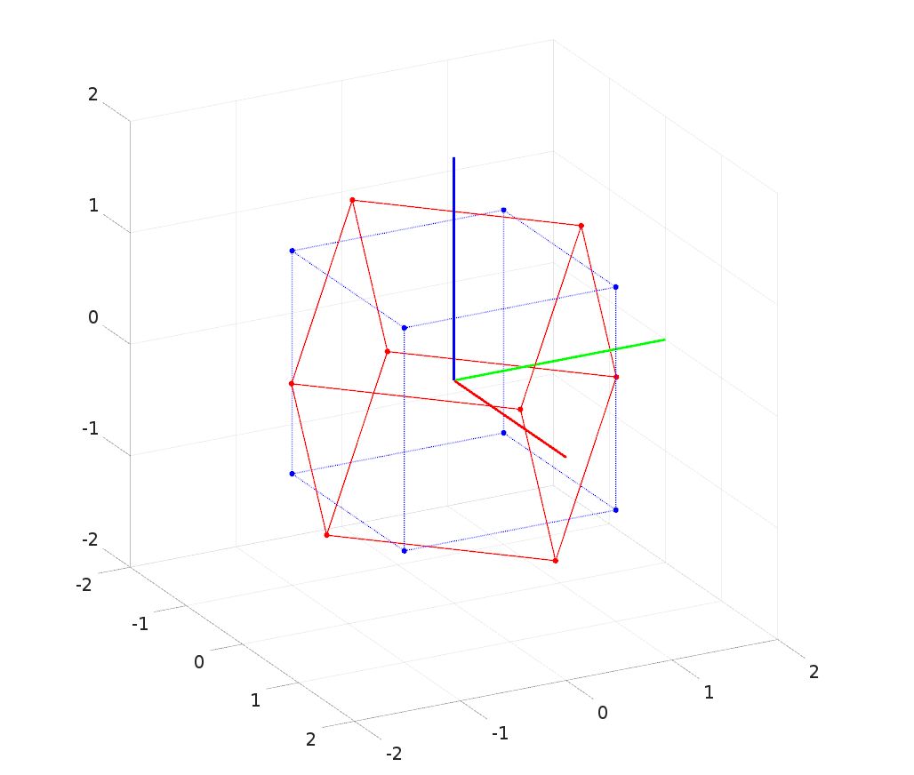
% Set up an array of points for a cube
pts = [1 1 1 1 -1 -1 -1 -1 ;
    1 1 -1 -1 1 1 -1 -1 ;
    1 -1 1 -1 1 -1 1 -1 ];

% Create the rotation matrices
theta_x = 45;
theta_y = 0;
theta_z = 30;

rot_x = [ cosd(theta_x), -sind(theta_x), 0; ...
          sind(theta_x),  cosd(theta_x), 0; ...
          0, 0, 1];

rot_y = [cosd(theta_y), 0,   sind(theta_y); ...
                     0, 1,               0; ...
        -sind(theta_y), 0,  cosd(theta_y)];

rot_z = [1, 0, 0; ...
          0, cosd(theta_z), -sind(theta_z); ...
          0, sind(theta_z),  cosd(theta_z)];

% Rotate the points
rot_pts = rot_x * rot_z * pts;

% Plot the axis marker
clf;
plot3([3 0],[0 0], [0 0],'r','linewidth',3);
hold on;
plot3([0 0],[3 0], [0 0],'g','linewidth',3);
plot3([0 0],[0 0], [3 0],'b','linewidth',3);


% Plot the vertices (original then rotated)
plot3(pts(1,:),pts(2,:),pts(3,:),'.b','MarkerSize',20);
plot3(rot_pts(1,:), rot_pts(2,:), rot_pts(3,:),'.r','MarkerSize',20);


% Plot the edges (original then rotated)
segment_order = [1,2;3,4;5,6;7,8;1,3;2,4;5,7;6,8;1,5;2,6;3,7;4,8];

for i = 1:size(segment_order, 1)
   plot3(pts(1,segment_order(i,:)), pts(2,segment_order(i,:)), pts(3,segment_order(i,:)), ':b');
   plot3(rot_pts(1,segment_order(i,:)), rot_pts(2,segment_order(i,:)), rot_pts(3,segment_order(i,:)), '-r');
end

% Clean up the view
axis equal;
axis(2*[-1, 1, -1, 1, -1, 1]);
view(60,20);

Bonus tips on working with 3D coordinate systems

The right-hand rules

In the world of engineering and physics there are quite a few "right-hand rules" (and some left-hand rules too). They are useful for various types of equations whose results have a specific direction. For example, they can tell us the direction that current will flow in a wire moving through a magnetic field, or the direction of the torque when a force is applied to a lever.

The two that we are concerned with here are shown below:

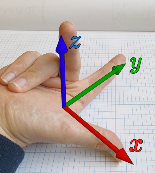
The first is the "normal" right hand rule for coordinate systems. It tells us what direction the $z$ axis should be, given the $x$ and $y$ axes. If you make a "finger gun" with your right hand, and don't fully bring your middle finger in but instead keep it perpendicular to the other two, you should be able to mimic the photo. Imagine that your thumb is the x axis, and your index finger is the y axis. Then, your middle finger would point in the direction of the z axis. If you imagine the standard x-y plane on a page, the axis extends "out of the page".

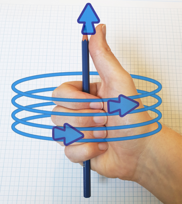
The second rule is the "grip" rule. It tells us what direction a positive rotation around an axis goes. If you make a "thumbs-up" with your right hand and imagine that your thumb is the direction that the axis points, the direction that your fingers point as they curl will be a positive rotation. Another way to think about this is that the positive rotation about one axis is the rotation required to turn the next axis into the one after that. For example if you look at the XYZ axis marker above, you can see that a positive X rotation can turn the Y arrow into the Z arrow. Likewise, a positive Y rotation could turn the Z arrow into the X arrow.

Be careful to remember to use your right hand! Although the maths will actually all work out if you use your left hand, you'll become very confused as all of your work will be incompatible with any existing code or tools that assume a right-handed system! The only exception to this is that some computer graphics systems (e.g. the Unity or Unreal engines) are actually based on a left-handed system and may require careful attention when converting.

Colours and models

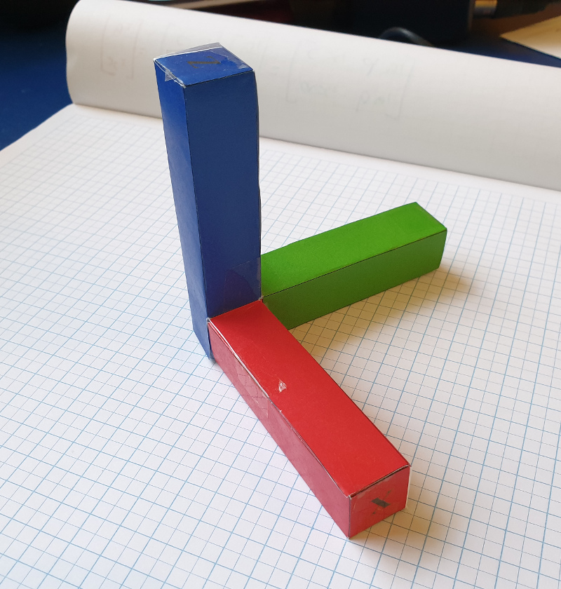
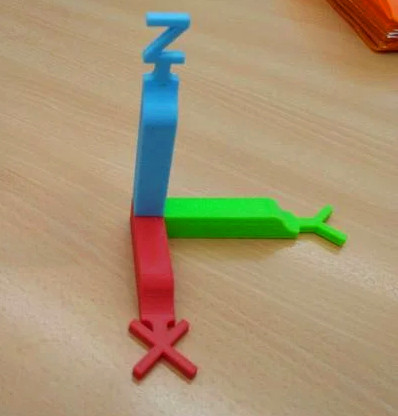
Another really useful tool in working with coordinate systems and being able to visualise them is to print out a model of one.

Extra Resources

• Wikipedia has an article on forming 3D rotation matrices by using multiple axial rotations.