Transformation Matrices
Combining our knowledge
So far we have learnt how to represent a pure rotation (including chained rotations) and a pure translation using matrices. In this post we'll look at a way to combine the two of these together into a single matrix representing both rotation and translation.
Mathematically, we want to represent the following function which takes a point and first rotates it around the origin, then translates it:
Although this function is not linear, it is still a special category of transformation called an affine transformation. This means it is a linear function (in this case ) with an offset (). In this post we'll explore in further depth the trick we used for translations, and how we can apply it to the more general problem of turning an affine function into a purely linear one.
Deriving the affine transformation matrix
What we're trying to do is turn the non-linear function above into a linear function in homogenous coordinates, just like we did in the last post. That is, we want to find a single matrix that can perform a rotation and translation together.
Augmenting our rotation matrix
The first step we need to take is to augment our rotation matrix to work on homogeneous coordinates. Like before, this means just adding an extra "1" to the end of each point vector.
We know (from our translation matrix) that the only way to get the 1 in the bottom row to carry through, is to set the bottom row to That leaves the two elements in the top-right corner. In order to prevent the "1" in the augmented point vector from affecting our rotation, both of these elements need to be 0, giving us:
So we have our rotation matrix in homogeneous coordinates, now we need to integrate the translational component.
Integrating the translation
In the last post we derived a "translation matrix" that performs a translation using homogeneous coordinates:
Now that we have a way to represent both rotations and translations in homogeneous coordinates, all we need to do to represent our affine transformation is to multiply them together!
One important thing to realise here is that we get a different result depending on whether we first rotate the point and then translate it, or vice versa. If we translate first, then our point will be in the wrong place to rotate (with respect to the origin), so it is important that the rotation happens first, i.e. .
So if we refer to our augmented rotation matrix as , and our translation matrix as we have the following:
Note that because matrix multiplication is associative, we can multiply and to form a new "rotation-and-translation" matrix. We typically refer to this as a homogeneous transformation matrix, an affine transformation matrix or simply a transformation matrix.
Examining T
Let's take a closer look at this structure of our transformation matrix. It's pretty clear that:
- The top left corner contains the original rotation matrix
- The top right hand corner contains the translation offset as a column vector
- The very bottom right hand corner contains a 1
- The rest of the bottom row (to the left of the 1) is all zeros.
We can simplify the representation of this matrix as shown below (note the use of a bold to indicate it is a zero vector).
This structure can be extended into 3D (or even higher dimensions) and will have the structure given below where is the number of dimensions.
It should also be clear that we can use this method with any affine transformation (things with the form ), not just when is a rotation matrix.
Summary of result
The point of all this is that we have taken our non-linear rotation-and-translation function and reworked it into a function which is linear in the new homogeneous coordinate system, .
Properties of transformation matrices
Chainability
Firstly, since our new affine transformation matrix is linear (using homogeneous coordinates), we are able to chain them together using multiplication, just like with the rotation matrices. What seemed pretty trivial at the time is now starting to become a pretty powerful tool. We can perform transform after transform and it all boils down to a few multiplications.
When we first looked at rotation matrices we saw that a rotation matrix multiplied by another rotation matrix produces a rotation matrix, in the same way a transformation matrix multiplied by a transformation matrix will always result in a transformation matrix.1
Inverse
The second useful property of the transformation matrix is that taking inverses is relatively easy. It's not quite as simple as the rotation matrix (where we simply had to take the transpose) but it's still pretty neat, which is great because in a few posts' time we'll start to use the inverse quite a lot!
The formula for the inverse of a transformation matrix is given below (without the derivation):
Note that if you are using this structure to represent other types of affine transformations (e.g. if you had a shear matrix instead of a rotation), you can still take advantage of this structure with the middle result, you just don't get the benefit of the easy inverse from the rotation matrix.
We can verify this property pretty easily:
What next?
Examples
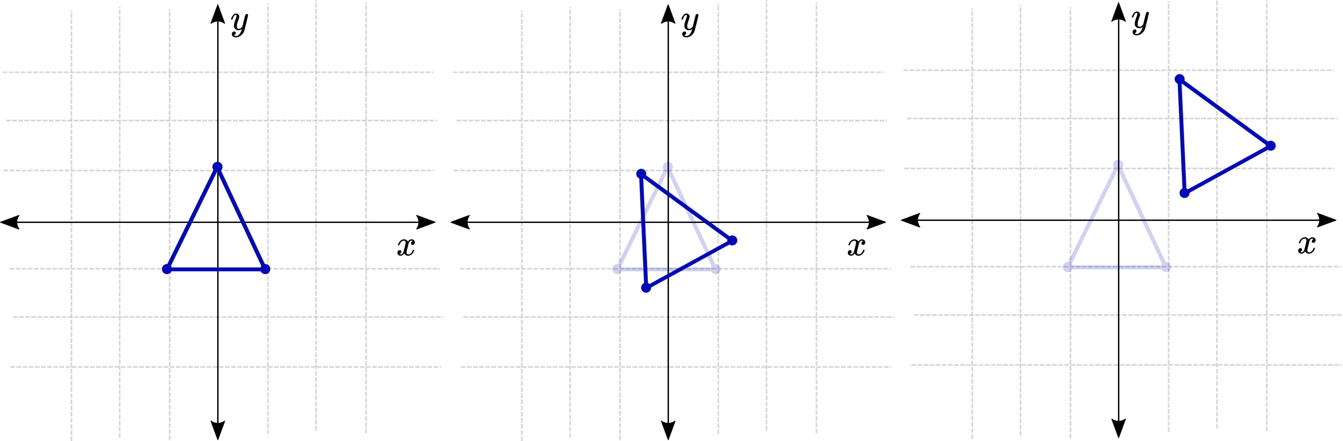
There are two examples given below. The first example shows the structure of the transformation matrix, and the effect of tweaking the different parts. The second demonstrates a very practical use case for a transformation matrix - plotting the corners of a robot as it moves along a trajectory through space.
Geogebra
In this example you can individually adjust the and translations, as well as the rotation angle, to see what effect it has on the resulting transformation matrix.
Loading
MATLAB/Octave
In this example, the transformation matrix is used to plot the path of a "robot" moving along the ground.
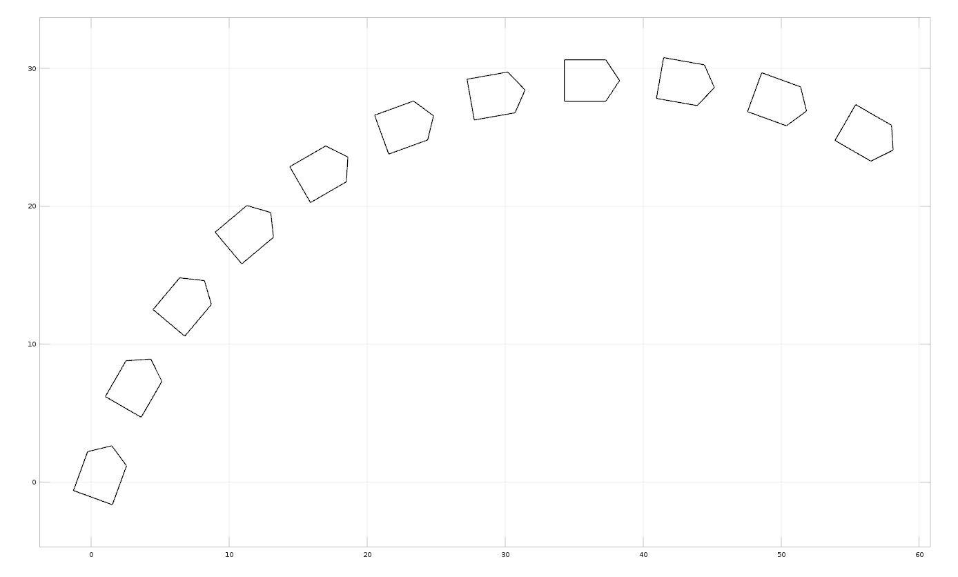
%% TRANSFORMATION TRAJECTORY DEMO
% Demonstrates the use of affine transformation matrices
% to plot an object moving along a trajectory

% Set up an array of points
x_points = [2, 2, 0.5, -1, -1, 2];
y_points = [-1, 2, 3,  2, -1, -1];
points = [x_points; y_points; ones(1, length(x_points))];

% Initial Conditions
sx = 0; sy = 0; theta = -20;

clf;
for t = 0:10
  % Compute the transformation matrix
  transf_mat = [cosd(theta), -sind(theta), sx; ...
                sind(theta),  cosd(theta), sy; ...
                           0,            0, 1];

  % Compute the new points
  transf_pts = transf_mat*points;

  % Plot the points
  plot(transf_pts(1,:), transf_pts(2,:), '-k' );
  hold on;

  % Update the state for the next plot
  sx = sx + 7*cosd(theta+90);
  sy = sy + 7*sind(theta+90);
  theta = theta - 10;
end

axis equal; grid on;
Extra Resources
- Wikipedia has an article on some of the more detailed mathematics behind affine transformations.
Footnotes
-
We noted in an earlier post that the set of all rotation matrices is technically known as the special orthogonal group, . Similarly, the transformation matrices are known as the special euclidean group, . Sometimes when we want to be explicit about what our variables mean, we write things like or which would be referring to a 2D rotation and transformation matrix respectively. The technical way of talking about this chaining process is to say that these groups are closed under multiplication, which means that if you take two things in that group and multiply them, the result will also be in the group. Another example of something closed under multiplication is the integers, you can never get a fraction by multiplying two integers. ↩